How to create a dynamic table in Excel
A simple table is quickly created in Excel, and using a few filters to sort the data is not a problem for most.
However, the function of having Excel generate a dynamic table from existing data is rarely used, as many do not really know what is possible with this option and what advantages it offers.
In this article, we would like to describe how you can turn static tables into dynamic ones, which possibilities and advantages a dynamic table offers, and also how you can convert them back into a normal static table.
1. Creating a dynamic table
1. Creating a dynamic table
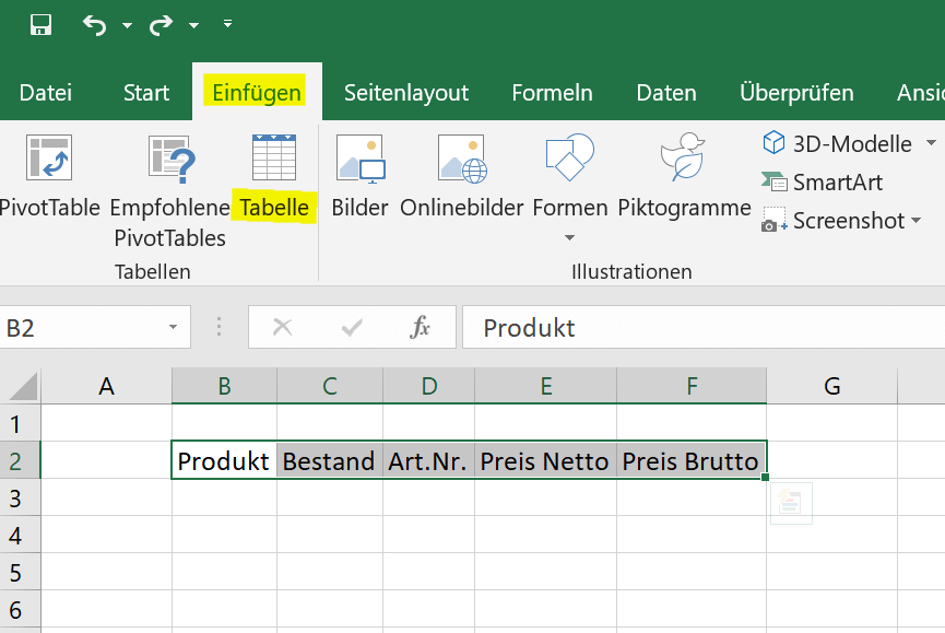
Creating a dynamic spreadsheet in Excel is actually very easy. You can do this by simply clicking in any cell and then on the “Insert” tab on “Table”.
Or you have already created a static table with headings and want to convert it to a dynamic table. To do this, simply mark the table area that is to be converted and then go to “Insert” and “Table”.
See fig.(click to enlarge)
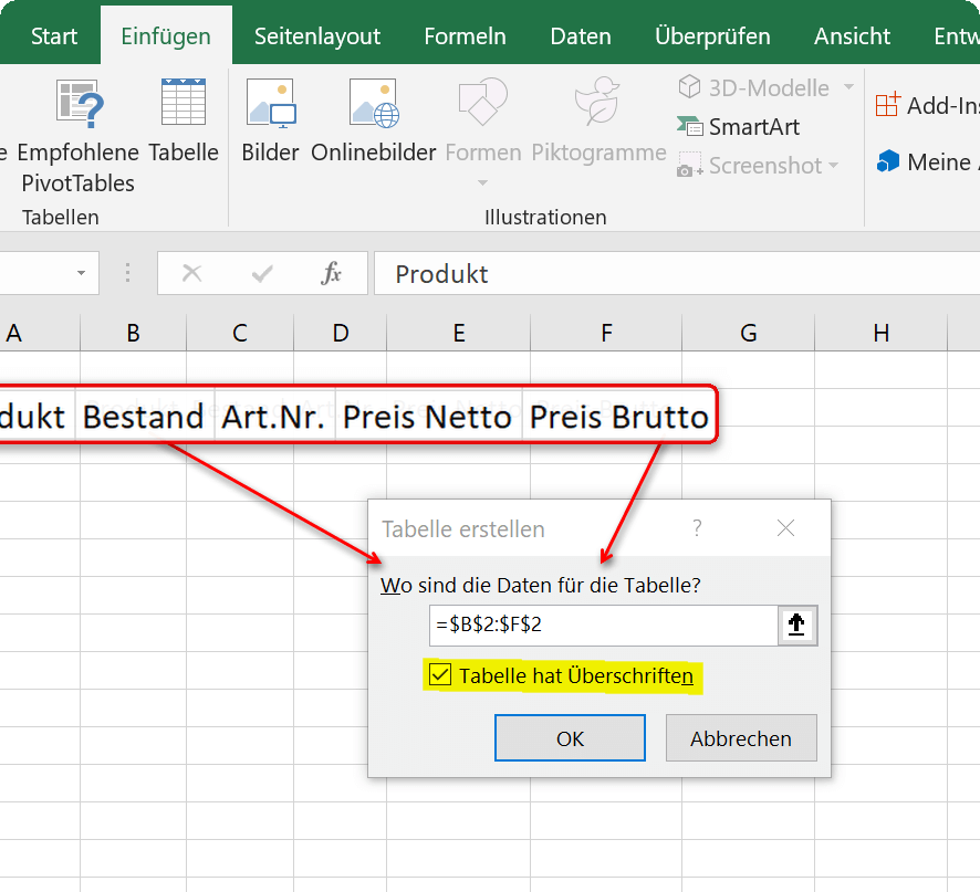
When you insert the table, you will also be asked whether the table has headings, and you may have to confirm this with a tick. If you already have headings, as in our example, you should also check the box, otherwise Excel will insert an additional line with column headings above your headings that is not required.
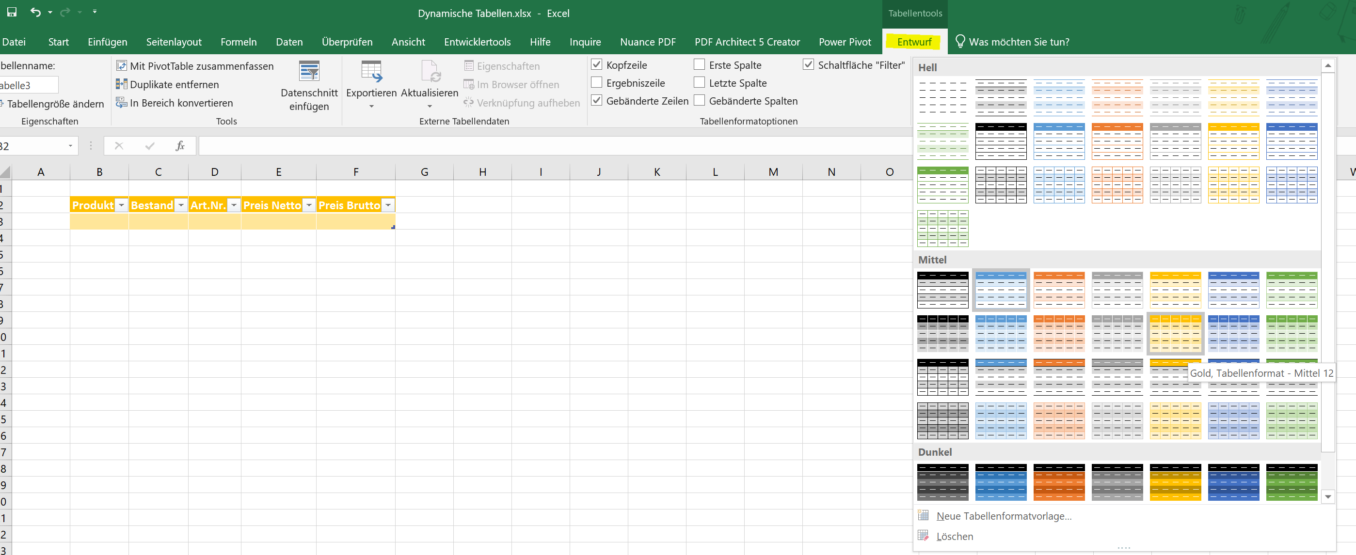
You can now change the dynamic table created in this way from one of the predefined color patterns in the layout, or you can also create your own color pattern. To do this, simply click in the table and then in the “Table Tools” – “Design” tab on the table format templates.
See fig.(click to enlarge)
2. Calculating with dynamic tables
2. Calculating with dynamic tables
With the newly created dynamic table, it is now also relatively easy to calculate.
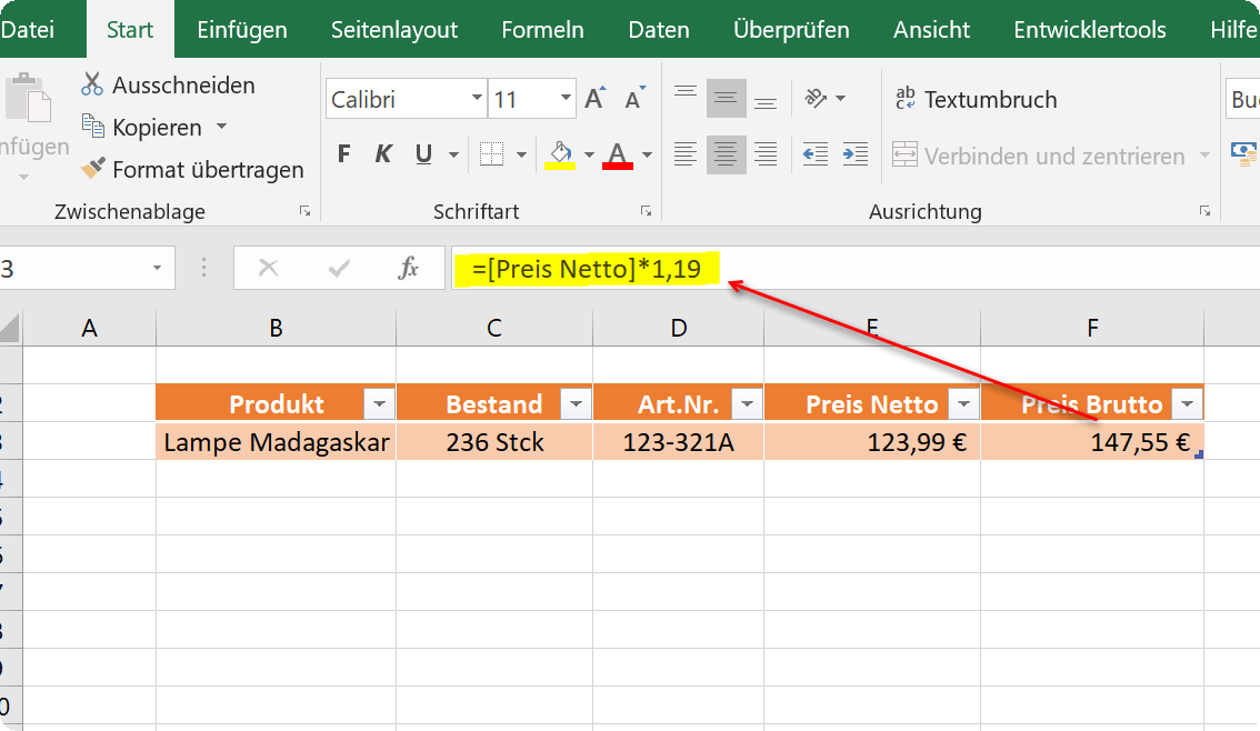
In our example, we simply created different products and calculated the gross price. To do this, we click in the cell in which the result should be and start with an “=”, as with any formula. Then we click in the first cell with the net price and multiply this value by 1.19 to calculate the 19% mark-up.
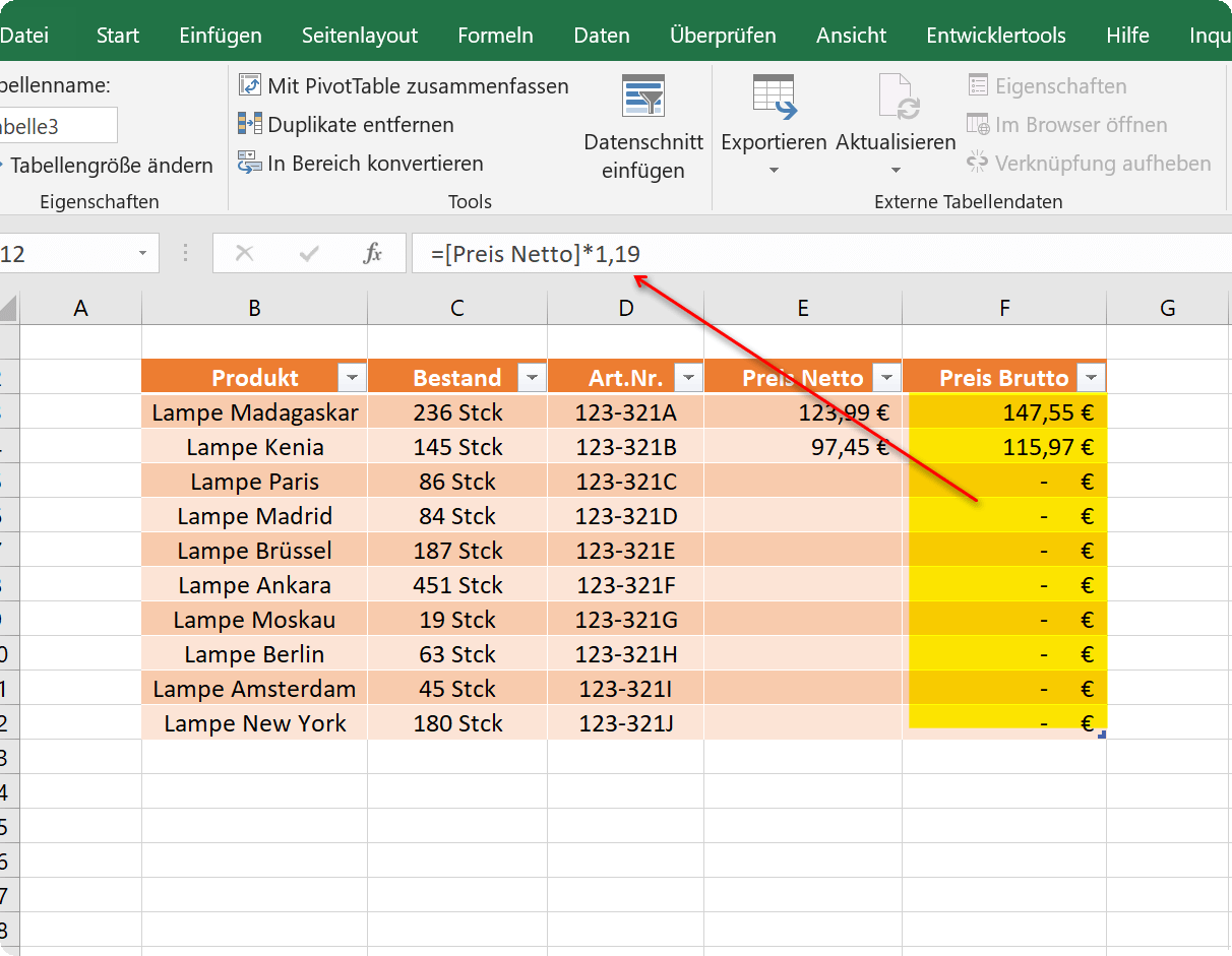
What is immediately noticeable in the formula bar is that the cell is not specified as the reference point, as in a static table, but the column heading. In this way, the formula in each new row for this area is inherited within the dynamic table, so that it does not have to be re-entered.
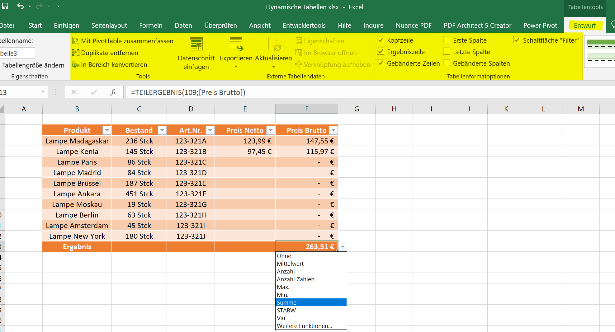
Of course, a table created in this way offers a number of other options and possibilities, which you can find in the “Design” tab under “Table tools”.
See fig.(click to enlarge)
A notice:
You can either extend the table by pressing the TAB key once in the last cell of the last row of the table, or you can simply drag down the lower right edge with the left mouse button.
3. Converting a dynamic table to a convertible range
3. Converting a dynamic table to a convertible range
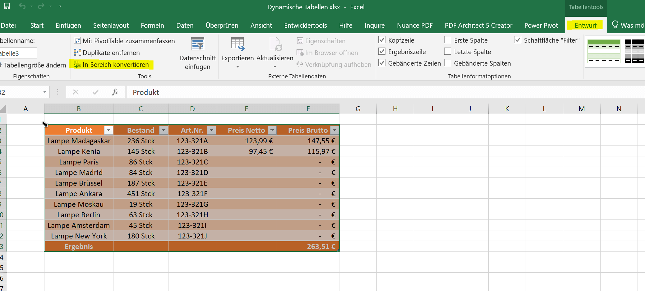
If at some point you want to convert the table back into a static table, you can do this again via the “Design” tab under “Table tools”. Simply select the entire dynamic table and then click “Convert to range”. You then only have to confirm a security query, and the dynamic table is resolved with all functions.
All previously created calculations are of course retained.
See fig.(click to enlarge)
Popular Posts:
Integrate and use ChatGPT in Excel – is that possible?
ChatGPT is more than just a simple chatbot. Learn how it can revolutionize how you work with Excel by translating formulas, creating VBA macros, and even promising future integration with Office.
Create Out of Office Notice in Outlook
To create an Out of Office message in Microsoft Outlook - Office 365, and start relaxing on vacation
The best backup solutions for your data
Keep your data safe and secure! Discover our best backup solutions for your valuable information now. Because safety is the be-all and end-all - and we have the perfect tips.
Internet Addiction – A serious look at a growing problem
Internet addiction is just as serious an illness as alcohol or drug addiction. Just that this is a mental illness. In this article we want to go into the phenomenon in more detail and provide assistance.
Main keyboard shortcuts in Windows 10/11
Entdecken Sie die wichtigsten Shortcuts in Windows 11, um Ihre Produktivität zu steigern. Von allgemeinen Befehlen bis hin zu spezifischen Fenster-Management- und System-Shortcuts, lernen Sie, wie Sie mit diesen Tastenkombinationen effizienter arbeiten können.
Encrypt USB stick – These options are available
Protecting sensitive data is essential. Encrypting USB sticks provides an extra layer of security. Whether it's built-in software, operating system features, third-party software, or hardware encryption, there are numerous options.

