How to create professional Excel invoice templates

Anyone who is very fresh in self-employment, sees himself at the beginning of all sorts of costs compared to the first in the start phase not come back through orders. Therefore you should save where it is possible. At the beginning you might not need a professional billing software, but you can invest it later if it works really well.

But even for employees who are currently still in a job, and the self-employed activity for the time being only incidentally, it is necessary to save costs where possible.

We would like to describe in this article how you can create your own invoice template in Microsoft Excel – Office 365 and send it as a PDF.

How to create professional Excel invoice templates

Anyone who is very fresh in self-employment, sees himself at the beginning of all sorts of costs compared to the first in the start phase not come back through orders. Therefore you should save where it is possible. At the beginning you might not need a professional billing software, but you can invest it later if it works really well.

But even for employees who are currently still in a job, and the self-employed activity for the time being only incidentally, it is necessary to save costs where possible.

We would like to describe in this article how you can create your own invoice template in Microsoft Excel – Office 365 and send it as a PDF.

1. Set up page and format

Before we begin to create a table in which the actual calculations are performed later, we should first adjust our sheet. Because just like a letter, our bill will also contain a letterhead with recipient, sender, etc.

And of course, the whole should fit into an envelope with window reasonable sense when you print it out and uses the usual zigzag fold.

As follows:

Open a new Excel document

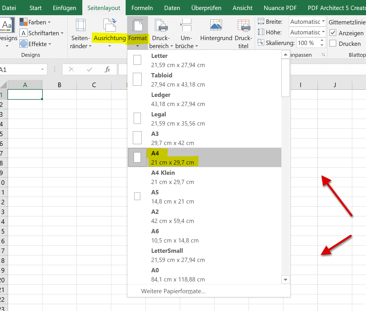
Use the “Page layout” tab – “Orientation” to select the portrait format

Then select “Format” DIN A4

After these first steps, your previously empty spreadsheet will be displayed with horizontal and vertical dashed lines, and you will know where the A4 sheet starts and where it ends.

It is now 10 columns (A – J) wide, and 50 rows high.

See picture: (click to enlarge)

Before we begin to create a table in which the actual calculations are performed later, we should first adjust our sheet. Because just like a letter, our bill will also contain a letterhead with recipient, sender, etc.

And of course, the whole should fit into an envelope with window reasonable sense when you print it out and uses the usual zigzag fold.

As follows:

Open a new Excel document

Use the “Page layout” tab – “Orientation” to select the portrait format

Then select “Format” DIN A4

After these first steps, your previously empty spreadsheet will be displayed with horizontal and vertical dashed lines, and you will know where the A4 sheet starts and where it ends.

It is now 10 columns (A – J) wide, and 50 rows high.

See picture:

2. Insert recipient and sender fields

Now it continues with the correct positioning for your logo, the statement INVOICE, the receiver and sender areas.

So that our content has some space to the edge reduce the column A (right mouse button / context menu) to 0.8 cm
Then mark the columns B to E and lines 1 to 4 and connect the cells via the tab “Start” – “Connect and center”

By way of example, we have already written in here “your company name / logo”.

Ultimately, you can simply write in your company name, or simply use the tab “Insert” – “Images” to create a previously created logo.

See picture: (click to enlarge)

Now we are preparing an area for the lettering “INVOICE”.

For this we mark the columns G to J and the lines 1 to 3, and connect them again. Here you can now from best beautiful large “INVOICE” write in, and center align.

Underneath we leave one line free, and continue in line 5 / column G with the details of the sender (your company), and write all the data into each other freely.

For clarity, I recommend under the information such as: name, address, etc. to release two lines, and then continue with the information: date of invoice, customer number, invoice number, tax or VAT number

Note: Do not worry if your details do not fit into a single cell, just override it. The grid lines that are visible in the standard, in any case, only a help, but will not be printed later.

See picture: (click to enlarge)

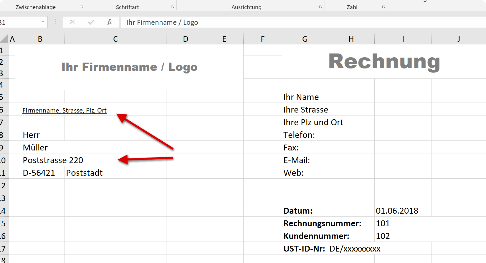
Next comes the area in the letterhead for the recipient address, as well as a small line in which the sender address is inserted again so that (even if undeliverable) the sender is visible without opening the letter.

To do this, insert the sender address in line 6 / column B, and optimally use a smaller font size (for example, 9 pt), and optionally underline this.

Then we release a row again, and continue in row 8 / column B and insert the recipient address there.

See picture: (click to enlarge)

Now it continues with the correct positioning for your logo, the statement INVOICE, the receiver and sender areas.

So that our content has some space to the edge reduce the column A (right mouse button / context menu) to 0.8 cm
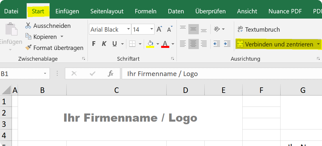
Then mark the columns B to E and lines 1 to 4 and connect the cells via the tab “Start” – “Connect and center”

By way of example, we have already written in here “your company name / logo”.

Ultimately, you can simply write in your company name, or simply use the tab “Insert” – “Images” to create a previously created logo.

See picture:

Now we are preparing an area for the lettering “INVOICE”.

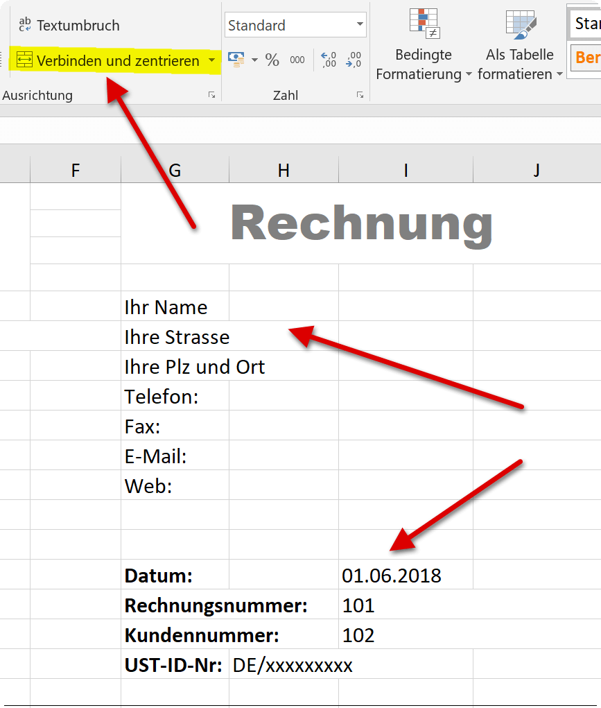
For this we mark the columns G to J and the lines 1 to 3, and connect them again. Here you can now from best beautiful large “INVOICE” write in, and center align.

Underneath we leave one line free, and continue in line 5 / column G with the details of the sender (your company), and write all the data into each other freely.

For clarity, I recommend under the information such as: name, address, etc. to release two lines, and then continue with the information: date of invoice, customer number, invoice number, tax or VAT number

Note: Do not worry if your details do not fit into a single cell, just override it. The grid lines that are visible in the standard, in any case, only a help, but will not be printed later.

See picture:

Next comes the area in the letterhead for the recipient address, as well as a small line in which the sender address is inserted again so that (even if undeliverable) the sender is visible without opening the letter.

To do this, insert the sender address in line 6 / column B, and optimally use a smaller font size (for example, 9 pt), and optionally underline this.

Then we release a row again, and continue in row 8 / column B and insert the recipient address there.

See picture:

3. Excel invoice template without tax card

Now that we have finished our letterhead, we can do the actual billing section.

For this we have now started in our example in line 21 / column B with the table. But this is not as crucial as it was with the letterhead, which will later fit into the window of an envelope. So, later on, you can do that a bit higher or lower, which suits you best.

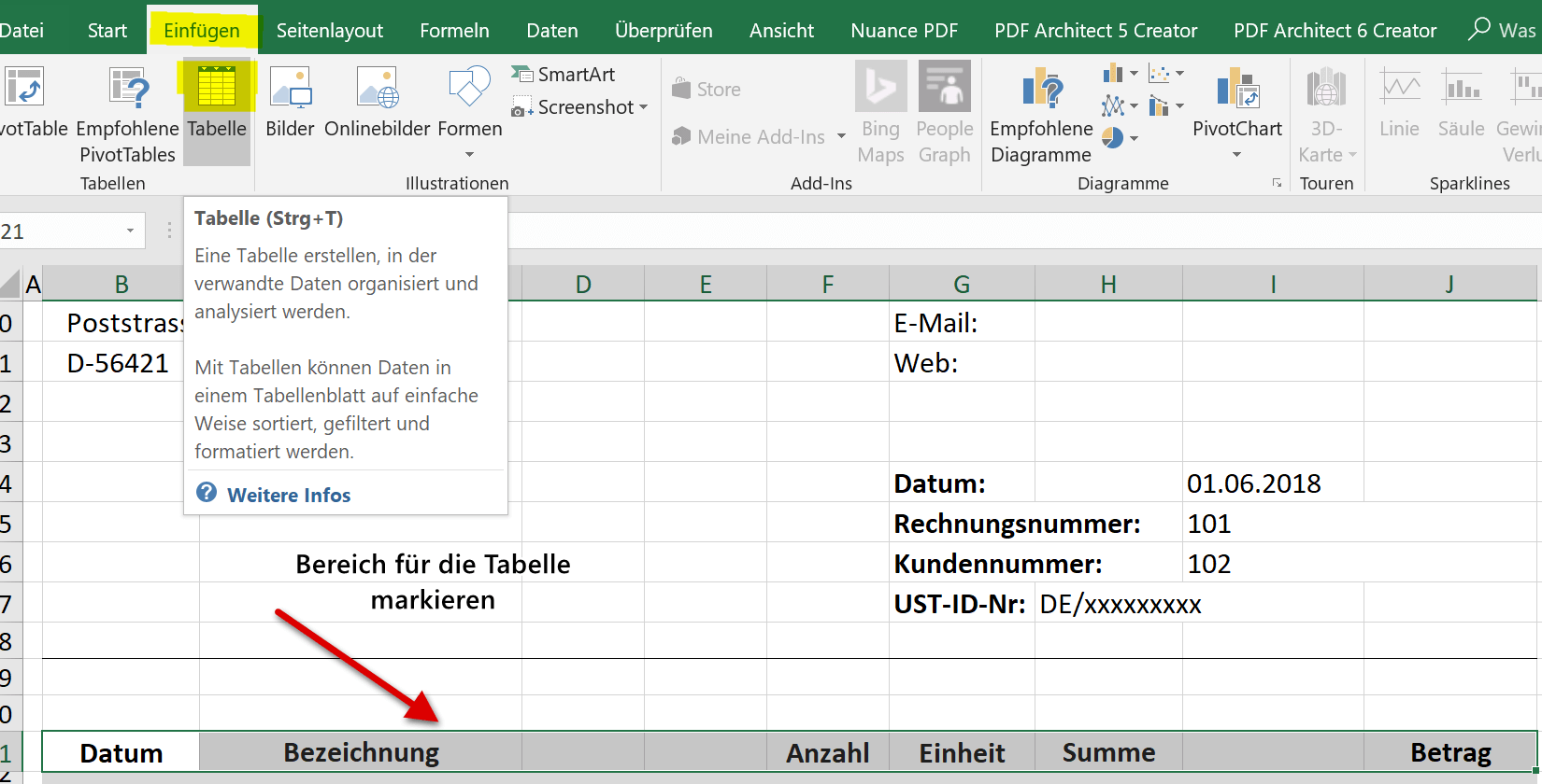
In line 21, we start in the horizontal with the entries for: date, description / specification, number, etc.

Then we mark all entries (keep the left mouse button pressed, and drag over)

Then continue via the “Insert” tab – “Table”

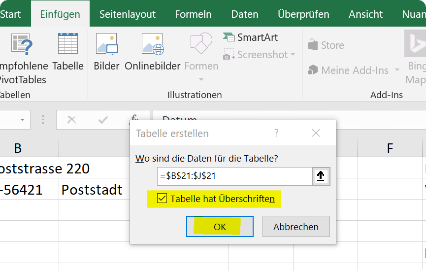
In the dialog box you will be asked again for the area in which the data for the table are (because you do not need to do anything, if everything is marked correctly)

The checkbox “Table has headers” must be selected

Confirm with OK

See picture: (click to enlarge)

The advantage of having a dynamic spreadsheet in Excel is that it makes it easier to insert computational operations and, as the name implies, can dynamically expand and update them.

You can now change the layout of your spreadsheet by selecting it and then using the “Table Tools” – “Design” – “Table Styles” tab either choose one of the templates or create your own.

However, you can change the layout at any time, without changing the functionality.

See picture: (click to enlarge)

Now you can easily expand the table either by pressing the TAB key in the last cell of the last row of the table, or optionally you have a small reinforcement at the bottom right of the table that you can just hold down (left mouse button pressed, and pull) and pull down.

This will always jump you directly to the next line

In the calculations within the table, we simply calculate the “hourly rate” x “number” in our example.
To do this, we go to the first row of the table under the “Amount” column and enter:

= SUM (F23 * H23)

and confirm with Enter

Note: This may of course be different in your formula depending on the division of rows and columns.

The function entered in this way is automatically updated for this column by Excel each time you expand the table by one line.

See picture: (click to enlarge)

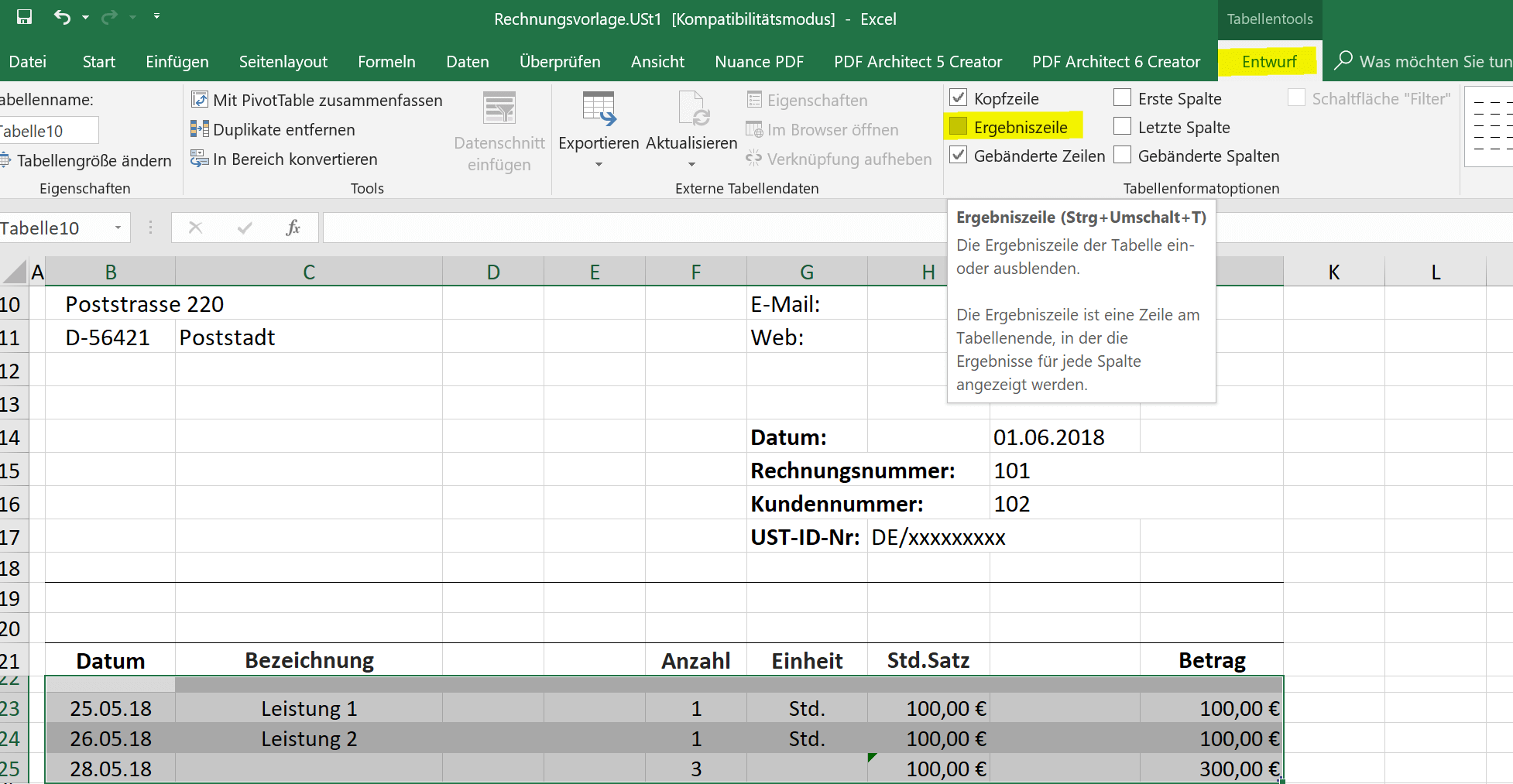
You can either integrate the now missing result row into the dynamic table by clicking in any cell of the table and then activate the check box “Result row” via the tab “Table tools” – “Design”.

The advantage of such a result row in a dynamic table is that it not only adds up sums, but also various other options such as: minimum, maximum, mean, and much more. get it done.

The disadvantage (at least with respect to our bill template) is that the result line is, of course, directly below the last line of our entries. It does not look so pretty, which is why we did not do it in our example, and instead just left one line empty, then made it a bit narrower, and then created a separate result line below it.

In this way, the whole thing does not look so squeezed, and the resulting row of results automatically slips one line lower with each extension of the table.

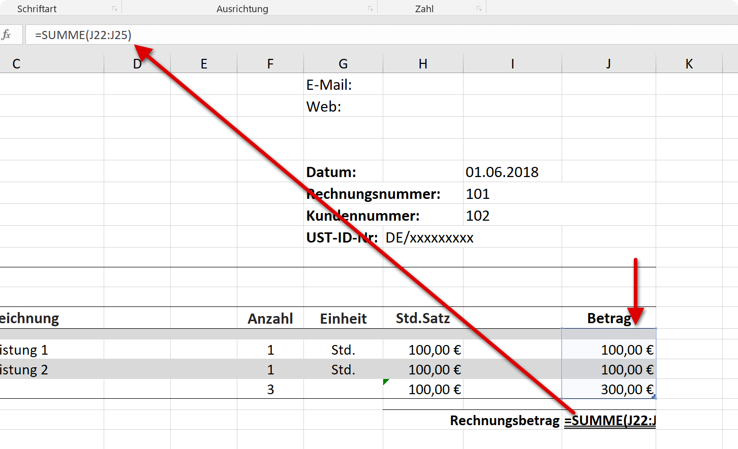
The calculation for our invoice amount we then simply make as follows:

mark the cell for the final invoice amount

enter = SUM (

mark the column area of the table with the added hourly rates

close the function again with a clip

See picture: (click to enlarge)

Now that we have finished our letterhead, we can do the actual billing section.

For this we have now started in our example in line 21 / column B with the table. But this is not as crucial as it was with the letterhead, which will later fit into the window of an envelope. So, later on, you can do that a bit higher or lower, which suits you best.

In line 21, we start in the horizontal with the entries for: date, description / specification, number, etc.

Then we mark all entries (keep the left mouse button pressed, and drag over)

Then continue via the “Insert” tab – “Table”

In the dialog box you will be asked again for the area in which the data for the table are (because you do not need to do anything, if everything is marked correctly)

The checkbox “Table has headers” must be selected

Confirm with OK

See picture:

The advantage of having a dynamic spreadsheet in Excel is that it makes it easier to insert computational operations and, as the name implies, can dynamically expand and update them.

You can now change the layout of your spreadsheet by selecting it and then using the “Table Tools” – “Design” – “Table Styles” tab either choose one of the templates or create your own.

However, you can change the layout at any time, without changing the functionality.

See picture:

Now you can easily expand the table either by pressing the TAB key in the last cell of the last row of the table, or optionally you have a small reinforcement at the bottom right of the table that you can just hold down (left mouse button pressed, and pull) and pull down.

This will always jump you directly to the next line

In the calculations within the table, we simply calculate the “hourly rate” x “number” in our example.
To do this, we go to the first row of the table under the “Amount” column and enter:

= SUM (F23 * H23)

and confirm with Enter

Note: This may of course be different in your formula depending on the division of rows and columns.

The function entered in this way is automatically updated for this column by Excel each time you expand the table by one line.

See picture:

You can either integrate the now missing result row into the dynamic table by clicking in any cell of the table and then activate the check box “Result row” via the tab “Table tools” – “Design”.

The advantage of such a result row in a dynamic table is that it not only adds up sums, but also various other options such as: minimum, maximum, mean, and much more. get it done.

The disadvantage (at least with respect to our bill template) is that the result line is, of course, directly below the last line of our entries. It does not look so pretty, which is why we did not do it in our example, and instead just left one line empty, then made it a bit narrower, and then created a separate result line below it.

In this way, the whole thing does not look so squeezed, and the resulting row of results automatically slips one line lower with each extension of the table.

The calculation for our invoice amount we then simply make as follows:

mark the cell for the final invoice amount

enter = SUM (

mark the column area of the table with the added hourly rates

close the function again with a clip

See picture:

4. Insert header and footer in Excel

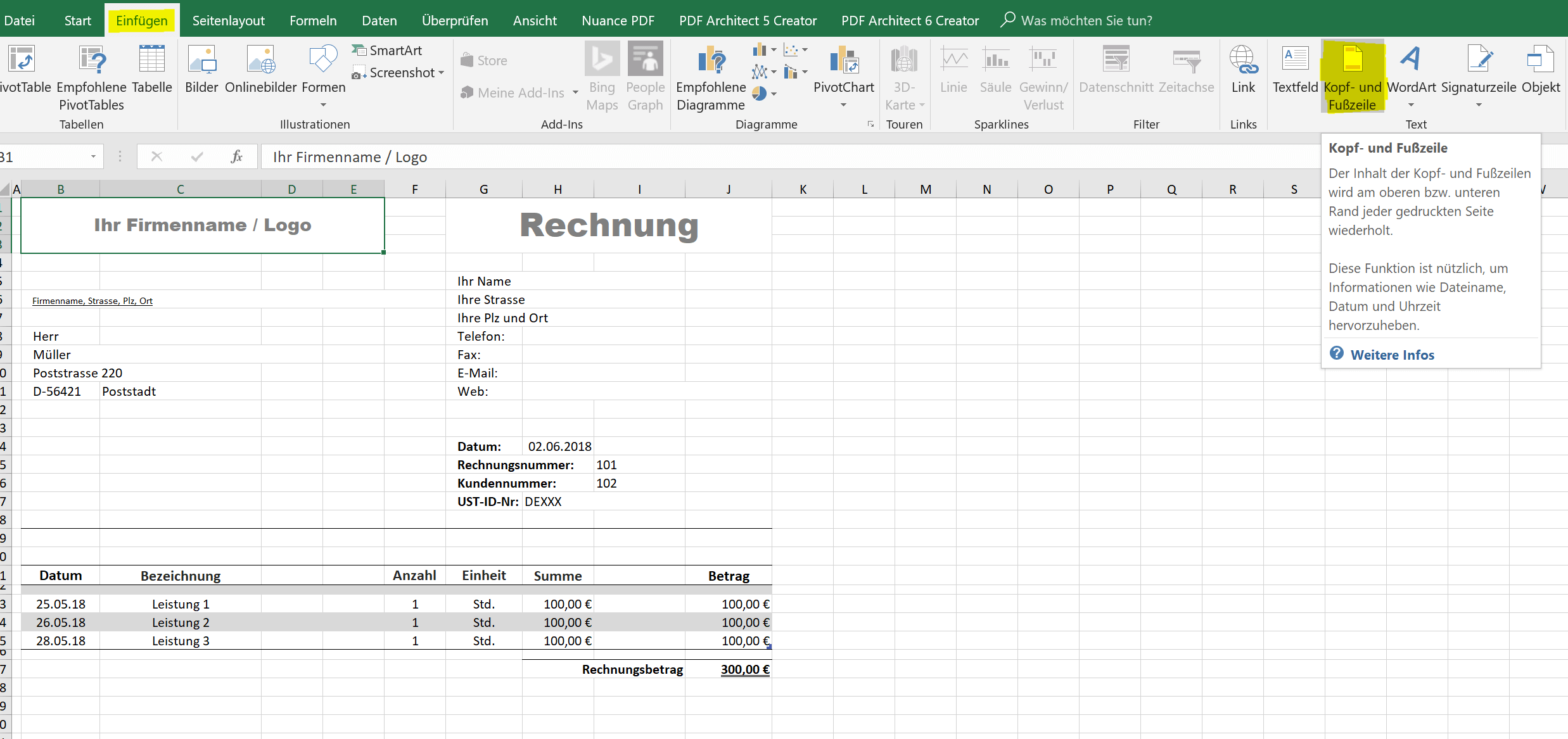
All that is missing now is the specification of our bank details, which we could just write anywhere under the billing area, but better something like this always looks in the footer of a document.

To do this, in the “Insert” tab, go to “Header and Footer”

See picture: (click to enlarge)

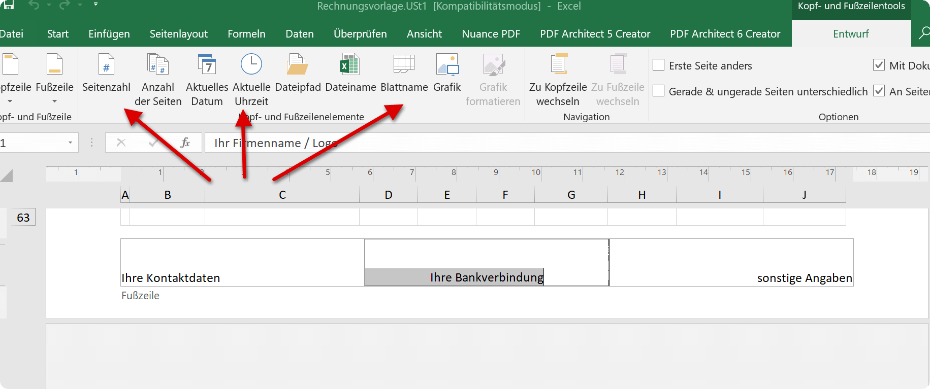
In the next window we will have different options of our footer to add the current day’s date and time, the respective page number, graphics, or own details (such as the bank details).

In this view, it is also easy to jump between the header and footer using the button

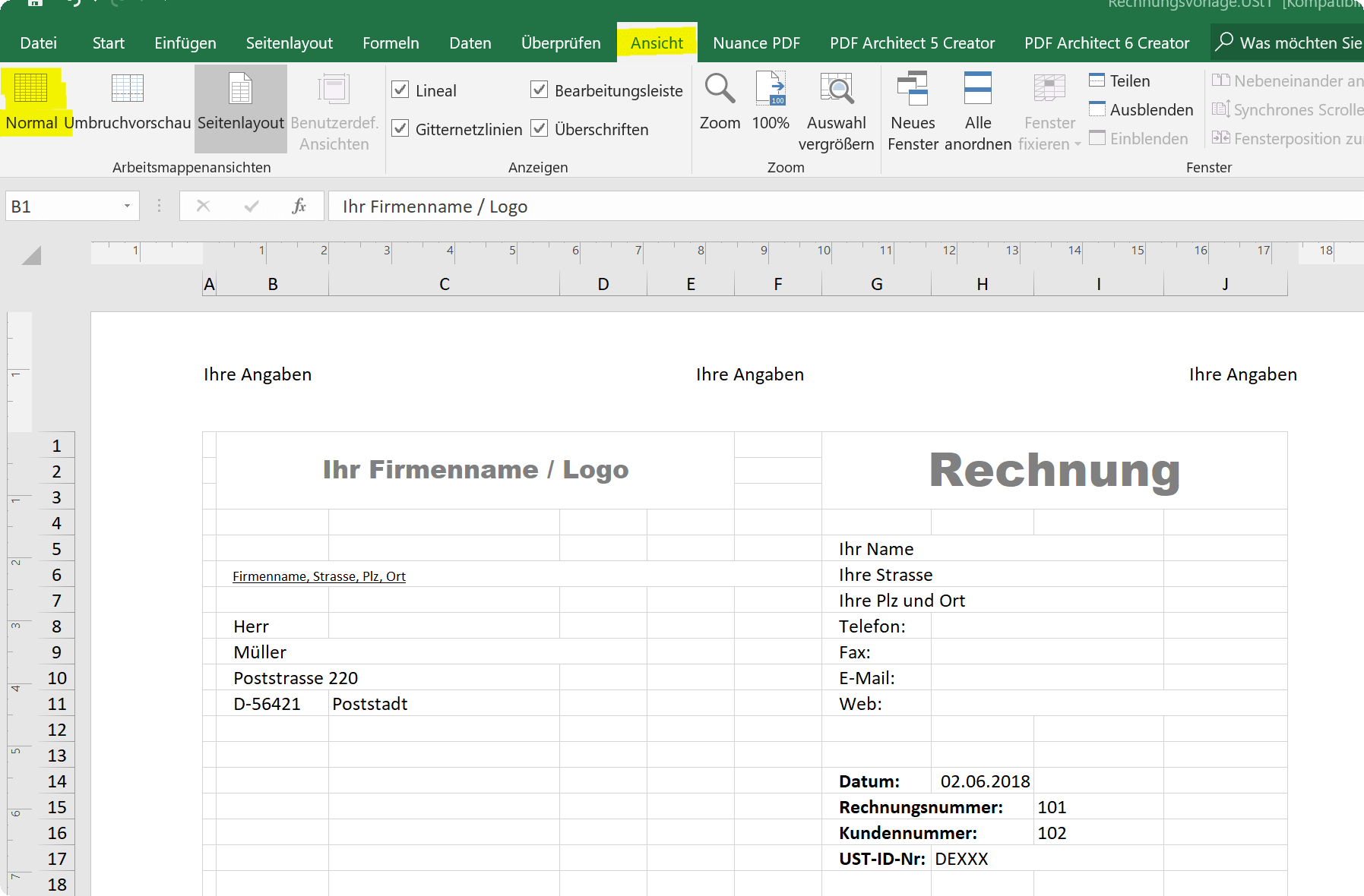
If you have entered your details there as desired, and want to return to normal view, just click in any of the bill templates outside the header and footer, and then in the View tab – Workbook Views – Normal.

See picture: (click to enlarge)

Note:
After you return to the normal view, the header and footer are no longer displayed. These are then only visible in the views “Page layout” and “Print view”.

All that is missing now is the specification of our bank details, which we could just write anywhere under the billing area, but better something like this always looks in the footer of a document.

To do this, in the “Insert” tab, go to “Header and Footer”

See picture:

In the next window we will have different options of our footer to add the current day’s date and time, the respective page number, graphics, or own details (such as the bank details).

In this view, it is also easy to jump between the header and footer using the button

If you have entered your details there as desired, and want to return to normal view, just click in any of the bill templates outside the header and footer, and then in the View tab – Workbook Views – Normal.

See picture:

Note:
After you return to the normal view, the header and footer are no longer displayed. These are then only visible in the views “Page layout” and “Print view”.

5. Excel invoice template with VAT card

If you have a sales tax identification number, then you are basically obliged to identify them in invoices.

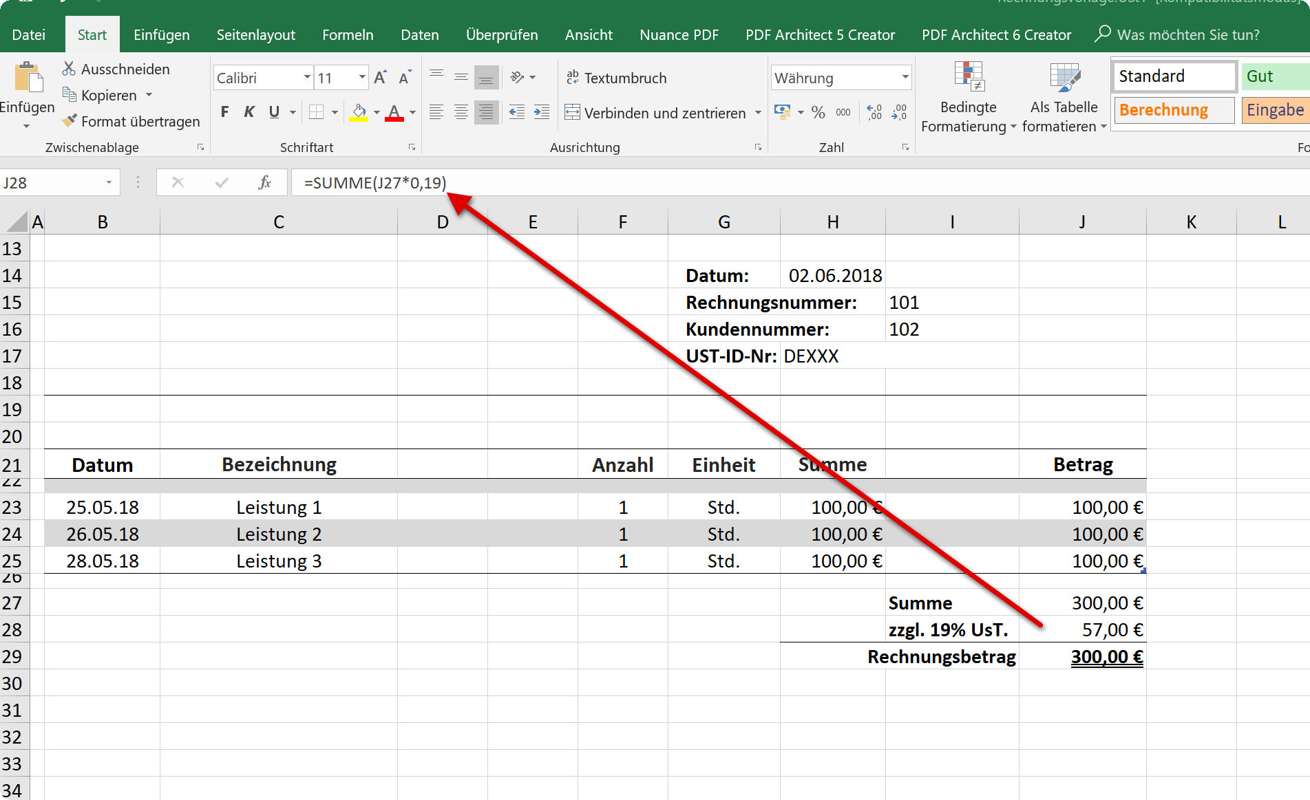
Thus, then the 100, – € in our example calculation would be our net amounts, and we have to show the 19% VAT separately, then to present them with the total net sum in our invoice amount as a gross amount.

This little extension is done relatively easily.

Just add two lines above the invoice amount

In the upper you can e.g. Enter sum, or net amount, and in the cell next to it just add the totals of the dynamic table (as before with the invoice amount)

And in the bottom line you wear e.g. plus 19% UsT. a, and in the cell next to it type the formula = SUM (J27 * 0.19)

In the cell Invoice amount you simply add both cells (net amount + UsT.)

See picture: (click to enlarge)

And that’s it.

You can now simply save the template as such in Excel, and then you can always use it again for new invoices.

Of course you will eventually resort to a professional billing and customer management, and this probably also to be able to better meet the legal documentation requirements, but for the beginning that is completely sufficient and above all free.

If you have a sales tax identification number, then you are basically obliged to identify them in invoices.

Thus, then the 100, – € in our example calculation would be our net amounts, and we have to show the 19% VAT separately, then to present them with the total net sum in our invoice amount as a gross amount.

This little extension is done relatively easily.

Just add two lines above the invoice amount

In the upper you can e.g. Enter sum, or net amount, and in the cell next to it just add the totals of the dynamic table (as before with the invoice amount)

And in the bottom line you wear e.g. plus 19% UsT. a, and in the cell next to it type the formula = SUM (J27 * 0.19)

In the cell Invoice amount you simply add both cells (net amount + UsT.)

See picture: (click to enlarge)

And that’s it.

You can now simply save the template as such in Excel, and then you can always use it again for new invoices.

Of course you will eventually resort to a professional billing and customer management, and this probably also to be able to better meet the legal documentation requirements, but for the beginning that is completely sufficient and above all free.

6. Save Excel spreadsheet as PDF

Finally, we should bring our invoices so created in a common format, which is also suitable to be sent by e-mail. Of course, the format of an Excel spreadsheet is not suitable at all.

So we just save it as PDF, or you can access a professional solution.

We can recommend here the program: Nuance Power PDF 2.0 >>>

This can be easily integrated into all Office programs at the time of installation, and offers a variety of options, such as: also converting PDF to Word, e-mails as PDF files, encryption, and much more.

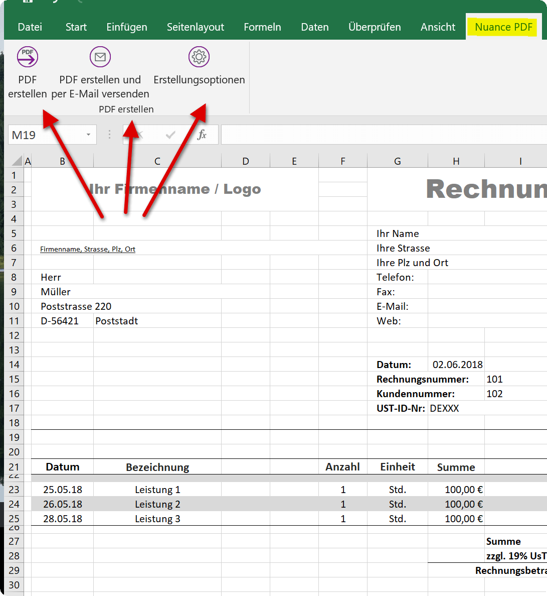
After the installation, you will always have an additional tab in every Office application that you can use to carry out a wide range of tasks.

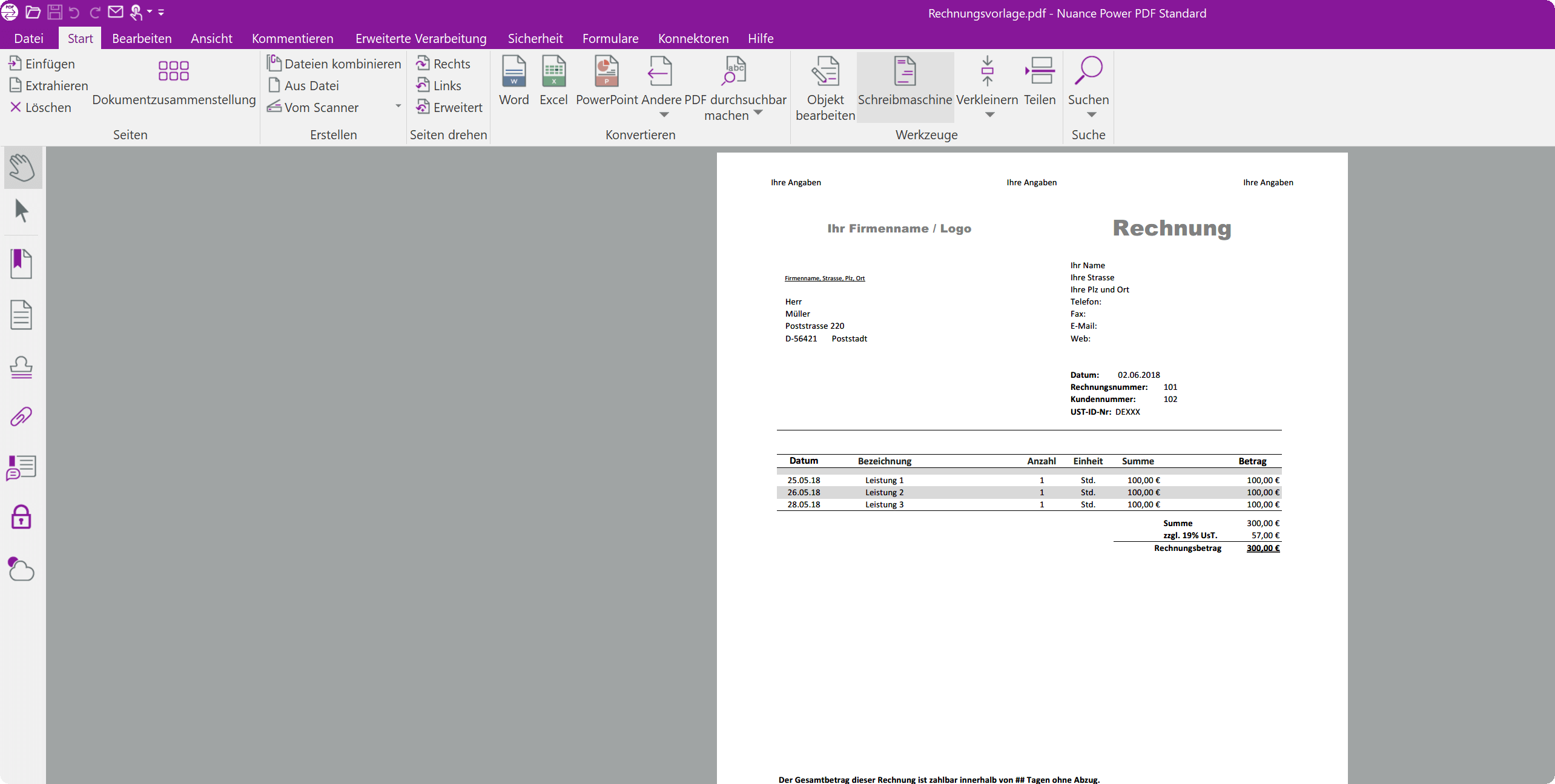
After saving as a PDF, we can then easily send the invoice as an attachment by e-mail to customers.

See picture: (click to enlarge)

Finally, we should bring our invoices so created in a common format, which is also suitable to be sent by e-mail. Of course, the format of an Excel spreadsheet is not suitable at all.

So we just save it as PDF, or you can access a professional solution.

We can recommend here the program: Nuance Power PDF 2.0 >>>

This can be easily integrated into all Office programs at the time of installation, and offers a variety of options, such as: also converting PDF to Word, e-mails as PDF files, encryption, and much more.

After the installation, you will always have an additional tab in every Office application that you can use to carry out a wide range of tasks.

After saving as a PDF, we can then easily send the invoice as an attachment by e-mail to customers.

See picture:

Zum Schluss sollten wir unsere so erstellten Rechnungen noch in ein gängiges Format bringen, welches sich auch eignet um per E-Mail versandt zu werden. Dafür eignet sich das Format einer Excel Tabelle natürlich überhaupt nicht.

Also speichern wir es einfach als PDF, oder man greift zu einer professionellen Lösung.

Empfehlen können wir hier das Programm: Nuance Power PDF 2.0 >>>

Dieses lässt sich bereits bei der Installation einfach in alle Office Programme einbinden, und bietet eine Vielzahl an Möglichkeiten wie z.B. auch das Umwandeln von PDF in Word, E-Mails als PDF archivieren, Verschlüsselung, uvm.

Nach der Installation haben Sie in jeder Office Anwendung immer einen zusätzlichen Reiter, über welchen Sie verschiedenste Aufgaben erledigen können.

Nach dem Speichern als PDF können wir die Rechnung dann ganz einfach als Anhang per E-Mail an Kunden versenden.

Siehe Abb.: