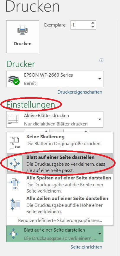
A common problem when printing Excel tables is that only part of the required content is printed out. Fortunately, this can be fixed relatively easily.

Solution:

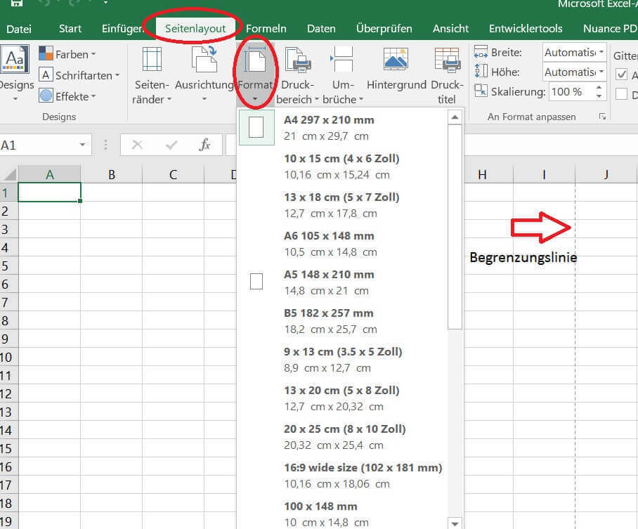
A great relief in the orientation of an Excel table is to make the page breaks visible

See fig. (Click to enlarge)

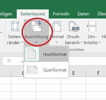
You can also choose whether you want the worksheet in portrait or landscape format. The boundary lines then also change according to the selection.

See fig. (Click to enlarge)

In the standard setting, everything that goes beyond this margin can no longer be seen in the printed area and is printed on a second page.

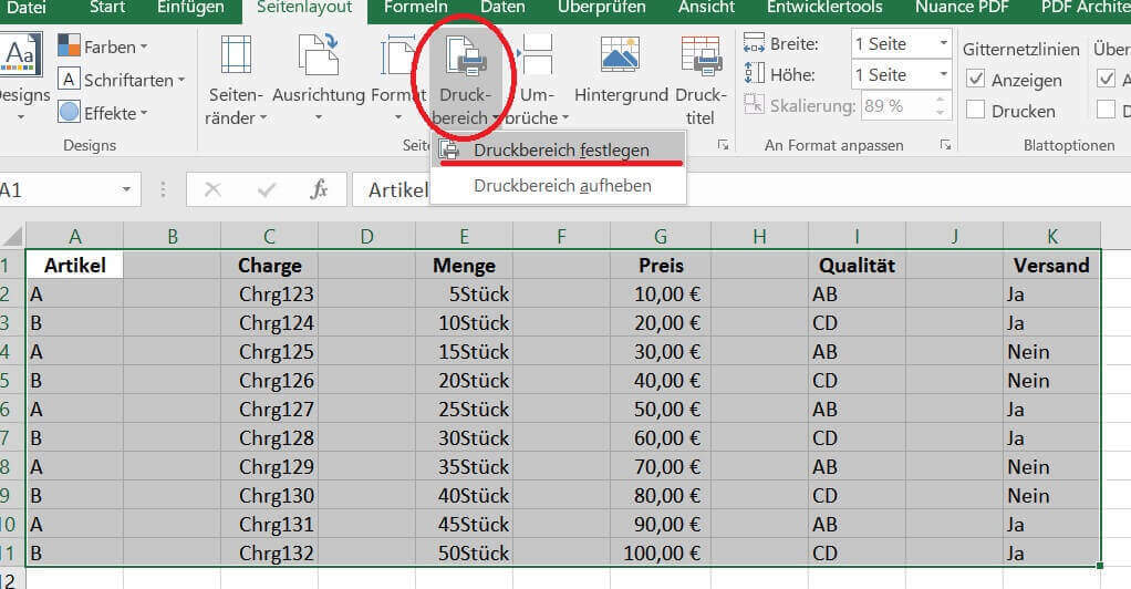
• So first of all we have to define the pressure range.
• To do this, we mark the entire area of the table that is to be printed out.

See fig. (Click to enlarge)

In the standard setting, everything that goes beyond this margin can no longer be seen in the printed area and is printed on a second page.

• So first of all we have to define the pressure range.
• To do this, we mark the entire area of the table that is to be printed out.

See fig. (Click to enlarge)

If you often create Excel tables (e.g. invoice templates) in which there is also a lot of text, you will at some point run into the problem that if the cells are automatically wrapped, the text is wrapped exactly where you can’t use it at all.

Solution:

• You can also edit all the text you enter in a cell in the formula bar.
• First mark the cell in which the text to be edited is located.
• Next, expand the field of view of the formula bar.

See fig. (Click to enlarge)

Now place the cursor directly in front of the first letter of the word which is to be broken into the next line. (In our example “in”)

See fig. (Click to enlarge)

• Now first press the “ALT” key and hold it down, and then the “ENTER” key.

Note:
You can break the text as often as you want and at any cell you want. However, if you later change the width and / or height of the cell, this can lead to undesirable results. You should only make these optical adjustments when the table is basically finished in terms of content.

If you have created an Excel table and would like to send the calculated results (e.g. by e-mail) to someone who may not be using Excel or an incompatible version for viewing purposes only. it can be helpful to convert these into the familiar PDF format beforehand.

Solution:
After you have created your table, do not just click save, as Excel usually uses the standard “xlxs” file format, but click “Save as” and then select the “PDF” file format

Tip:
The easiest way to get to the save options is to press the “F12” key directly from the worksheet.

If you have created an Excel spreadsheet, it is often saved on a drive (e.g. in a network) to which many people within this network have access. However, not everyone should have access to all files in this drive.

It can therefore be helpful to protect certain files from unauthorized access with a password.

Solution:

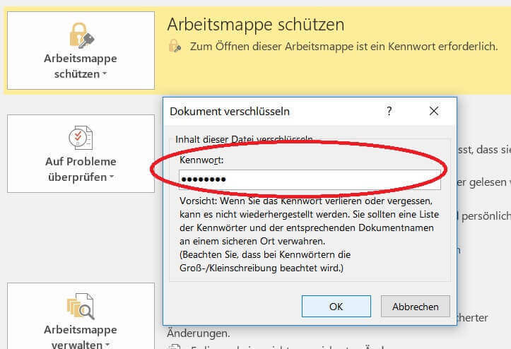
After you have created your tables in a workbook, go to: “File / Information / Protect workbook” to the point: “Encrypt with password”

See fig. (Click to enlarge)

Here you can now assign any password that will be required later to open the file.

Please make a careful note of the password, otherwise you will no longer be able to open the file without this password!

See fig. (Click to enlarge)

Note:
The file is still visible to everyone, but the workbook can only be opened with the valid password (case-sensitive).

Since Excel is a spreadsheet and not a word processing program, it is a bit difficult for some entries that have to do with text to implement them as the user would like.

Example:
You want to enter the following text in a cell: “= the value of:”

The problem that will now occur after you have entered the equal sign and your text and confirmed with Enter is that Excel assumes that you want to enter a formula, since all formulas in Excel now begin with an “=” sign. The following error message then appears: “#Name?”

Solution:
In the cell in which you want to start with the “=” sign, insert an invisible apostrophe beforehand with the key combination “ALT GR” + “apostrophe (´)”. This is not displayed and also not printed.

Note:
This procedure can be applied to all mathematical signs such as +, -, / etc.

Anyone who has ever created an extensive Excel table with a lot of calculations knows that at some point there will come a point where you no longer know exactly in which cells calculations were made and where numbers were entered manually.

Wouldn’t it be helpful to know in which cells there are formulas?

Solution:
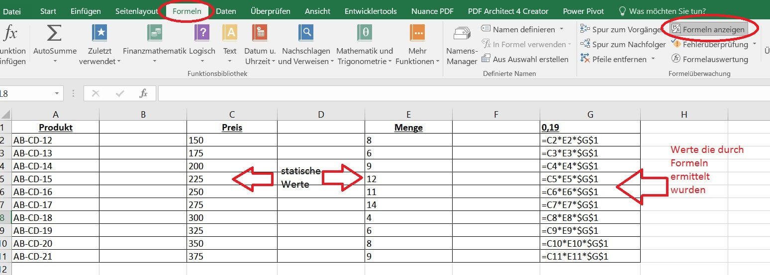
Select under the register: “Formulas” / “Show formulas”

See fig. (Click to enlarge)

Here you can now see exactly where formulas are stored in your worksheet.

When you have created a table with some calculations and cell references, you can, as already shown in tip 6, display the cells where formulas are stored.

However, the longer a formula is, the more strenuous it is to look for the cells specified there on the sheet and to find an error. Wouldn’t it be practical if the trace that led to the calculation could be displayed?

Solution:
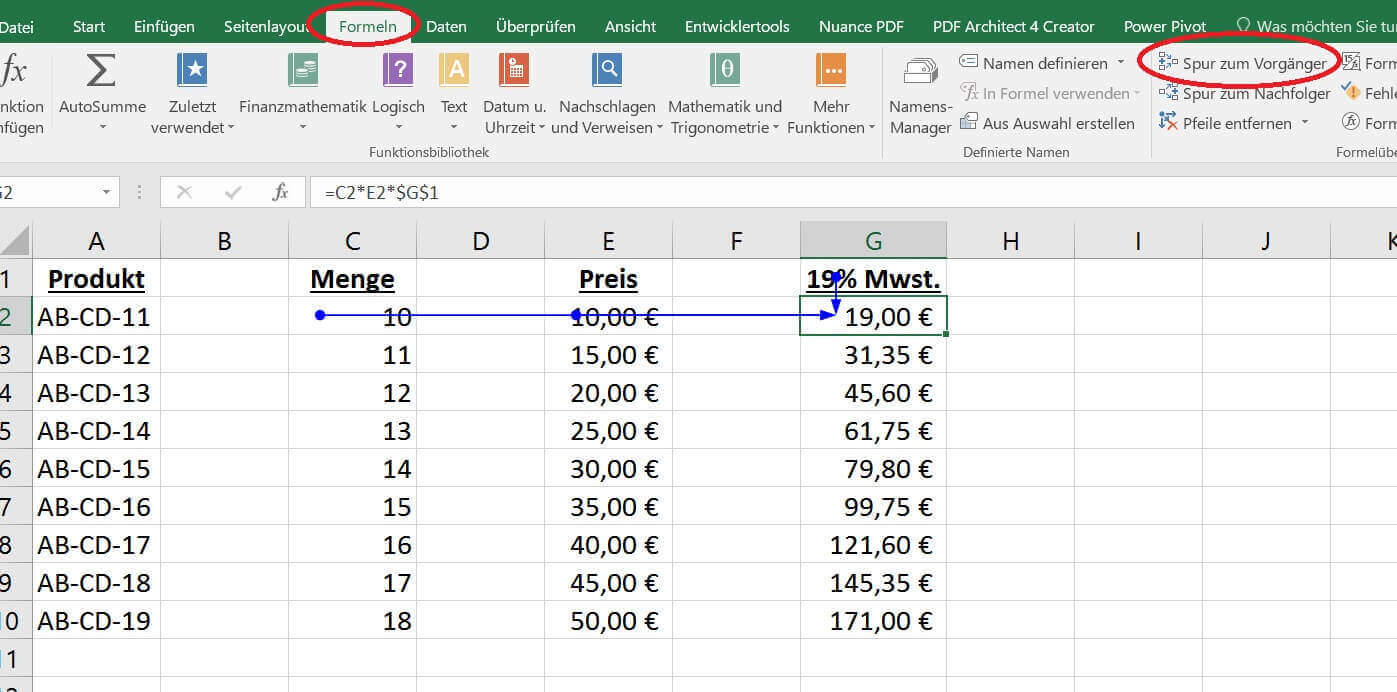
Select a cell in which Excel calculations were carried out, and then select in the register: “Formulas” / “Track to predecessor”

See fig. (Click to enlarge)

Here the arrows show you with which cell values the result in the marked cell came about.

Note:
If too many cell references have flowed into the result of a cell, it will of course become confusing again with all the arrows, but this tip can be quite helpful for smaller calculations.

If you have created a table and you share it with others (e.g. in a network) and you should only be able to edit certain areas, but the rest of the table can only be changed by yourself, you should write-protect these cells .

Solution:
Basically, all cells in Excel are marked with “Locked” in the formatting. This means that if you now write-protect the worksheet, nothing can be changed at all.
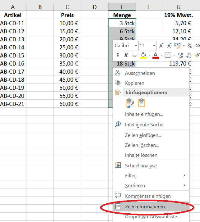
First, mark all cells or cell areas that should later be able to be changed by all employees who have access to the file.
Then activate the context menu over the marked cells with the right mouse button and select “Format cells”.

See fig. (Click to enlarge)

Next, go to the “Protection” tab in the cell formatting menu, and remove the tick “Locked”.
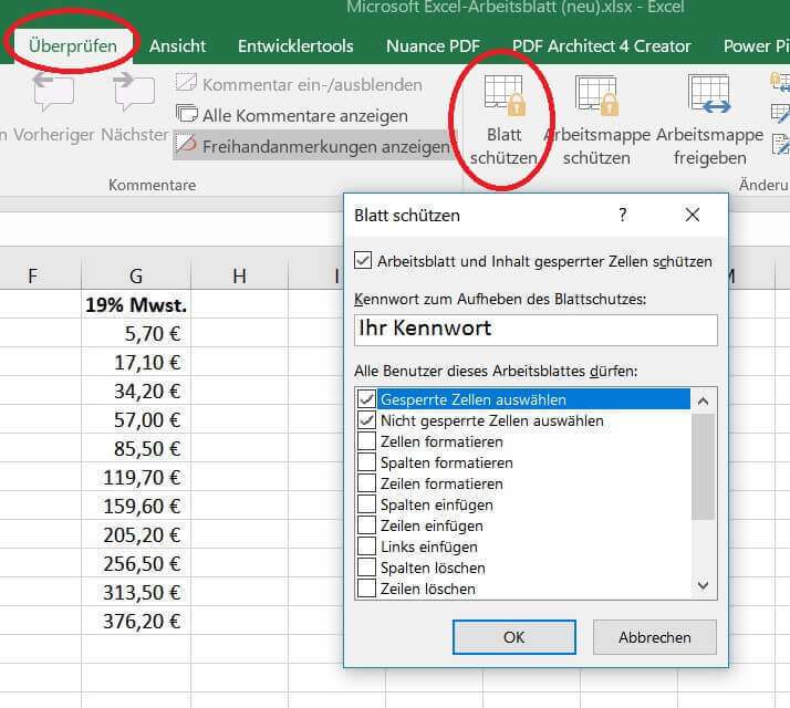
In the last step, we go to “Protect sheet” under the “Check” tab and assign a password there (optionally), and check the respective checkmarks for the processing restrictions that we would like to assign to these cells.

See fig. (Click to enlarge)

Popular saying goes that if you don’t make mistakes, you don’t work either. And there is actually something to this wisdom. Because it just happens that you just “clicked” yourself at a certain point, and suddenly everything looks completely different than it did a second ago. Fortunately, Excel 2016 allows you to undo up to 100 work steps.

Solution:
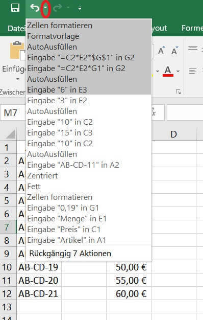
In the upper area of the worksheet (directly above the “Start” tab) go to the small arrow pointing downwards, and you can see the last work steps made there.

Now select from the list of the last work steps displayed how many steps you want to undo.

See fig. (Click to enlarge)

Note:
In most cases, the mistake is immediately identified and you want to reverse it quickly. In this case, just use the following keyboard shortcuts:

• “CTRL” + “Z” (undo last step)
• “CTRL” + “Y” (one more step forward)

Especially with somewhat longer tables, it makes perfect sense to fix the top line of a table so that it remains constantly visible.

You can do this very simply by selecting “Fix top line” in the “View” tab – “Fix window”.
But then only the top line is fixed and remains permanently visible.

Another variant that can sometimes be useful is that an entire area remains permanently displayed. But you can basically just as easily reach this via the above-mentioned path. The only difference is that instead of “Fix top line” simply “Fix window” is selected.

The position of the cursor (the currently selected cell) is decisive for fixing a window. The window is fixed from exactly this cell to the left and upwards.

See fig .: (click to enlarge)