Excel Tutorial: How to quickly and safely remove duplicates
Anyone who works with lists knows the problem: email distribution lists, customer lists, or order data are often “polluted” and contain duplicate entries. These duplicates distort analyses and create chaos.
Fortunately, Excel has a built-in function that solves this problem in seconds.

A practical example: An order list
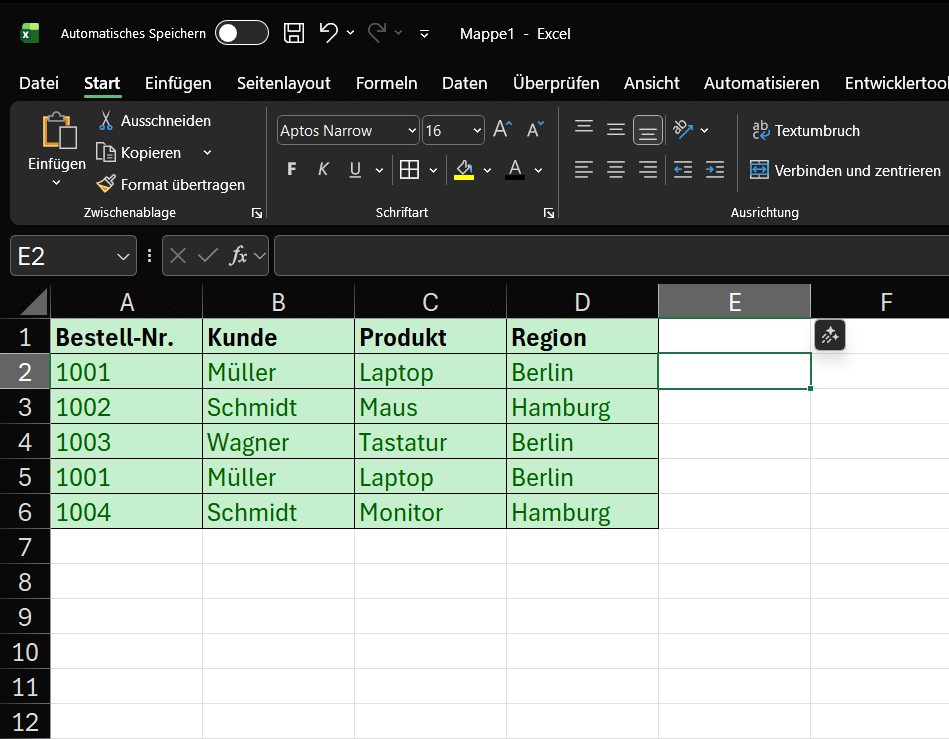
Imagine we have the following table with order data. We immediately see that some entries are repeated.
Our example data (range A1:D6):
Goals:
- Goal A: We want to remove exactly identical rows (row 5 is a duplicate of row 2).
- Goal B: We want to obtain a unique list of all customers (Müller, Schmidt, Wagner).
Step-by-step instructions: How to remove duplicates
The “Remove Duplicates” function permanently deletes data.
⚠️ Important Security Note: Before you begin, always copy your worksheet or create a backup of your file. This way, if you make a mistake, you can revert to the original.
Step 1: Select the Data Range
- Click in your data table. Excel usually detects the contiguous range automatically. However, the safest method is to manually select the entire range (in our example, A1:D6) with your mouse.
Step 2: Finding the Function
- Go to the “Data” tab in the ribbon.
- Find the “Data Tools” group.
- Click the “Remove Duplicates” icon.
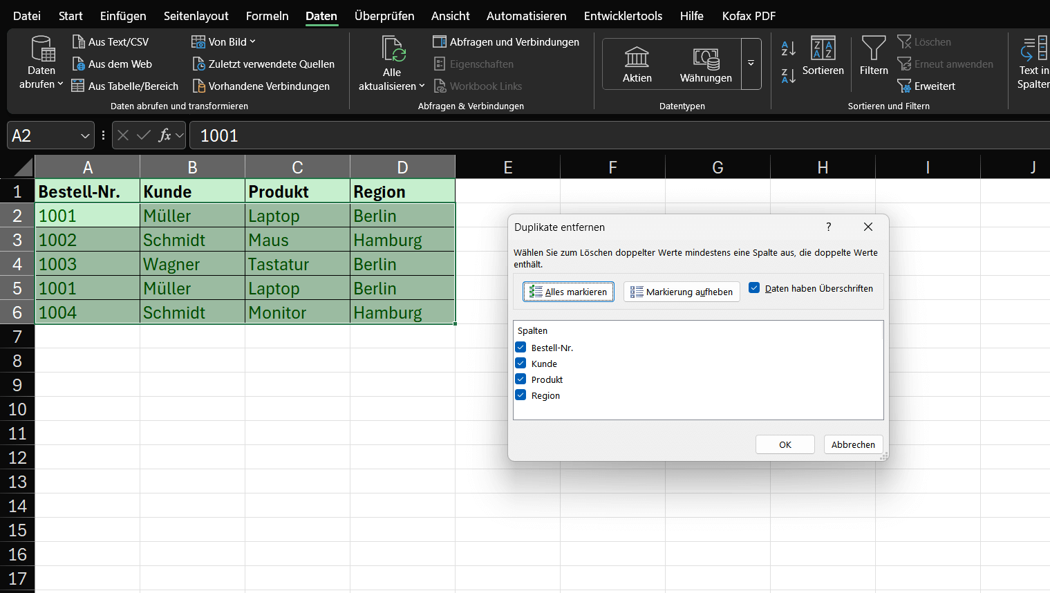
Step 3: The Dialog Box (The Most Important Step)
- A small window will open. This is the control center for the deletion process.
- “Data has headers”: Since our table has headers in row 1 (Order No., Customer, etc.), be sure to leave this checkbox selected. Excel will then ignore this row when deleting.
- Columns: Here, Excel lists all the columns from your selection.
… This is where Excel decides what it considers a “duplicate”.
The two scenarios (Goal A vs. Goal B)
Scenario A: Deleting Exactly Identical Rows
Goal: We want to delete only row 5, as it is identical to row 2 in every column.
- Open “Remove Duplicates” (as described in steps 1 & 2).
- In the dialog box (step 3), ensure that ALL columns (Order No., Customer, Product, Region) are checked.
- Click “OK”.
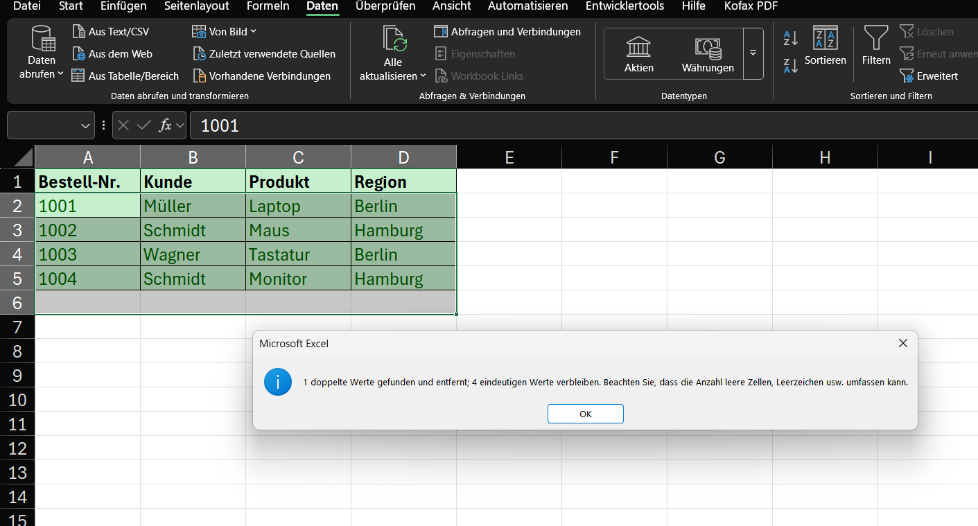
Result: Excel compares entire rows. Since only row 5 is an exact match for row 2, it is deleted. Excel reports: “1 duplicate found and removed; 4 unique values remain.”
Note: Row 6 (Schmidt, Monitor) is NOT deleted, as it differs (in the product field) from row 3 (Schmidt, Mouse).
Scenario B: Creating a unique list based on ONE column
Goal: We are not interested in the entire table. We only want a unique list of all customers (Müller, Schmidt, Wagner).
- Open “Remove Duplicates”.
- In the dialog box, first click “Deselect” to remove all checkmarks.
- Check only the column you want to check for uniqueness – in our case, “Customer”.
- Click “OK”.
Result: Excel only looks in column B.
- Row 2 “Müller” is kept.
- Row 3 “Schmidt” is kept.
- Row 4 “Wagner” is kept.
- Row 5 “Müller” (duplicate!) is deleted.
- Row 6 “Schmidt” (duplicate!) is deleted.
- Excel reports: “2 duplicates Found and removed; 3 unique values remain.
💡What happens: Excel always keeps the first entry it finds in the list and deletes all subsequent duplicates (based on the selected columns).
Summary (Pro tips)
Make a backup: Always copy the worksheet first!
- All columns = Deletes only rows that are completely identical.
- One column = Creates a unique list based on this one column (e.g., listing all customers only once).
Caution: This function deletes the entire row. If you select only “Customer” in Scenario B, the associated order data (laptop, mouse, etc.) will also be deleted. If you don’t want this, copy the customer column to a separate area first and apply the function only there.


Beliebte Beiträge

More than just a password: Why 2-factor authentication is mandatory today
Why is two-factor authentication (2FA) mandatory today? Because passwords are constantly being stolen through data leaks and phishing. 2FA is the second, crucial barrier (e.g., via an app) that stops attackers – even if they know your password. Protect yourself now!

Beware of phishing: Your PayPal account has been restricted.
Beware of the email "Your PayPal account has been restricted." Criminals are using this phishing scam to steal your login information and money. They pressure you into clicking on fake links. We'll show you how to recognize the scam immediately and what to do.

Excel Tutorial: How to quickly and safely remove duplicates
Duplicate entries in your Excel lists? This distorts your data. Our tutorial shows you, using a practical example, how to clean up your data in seconds with the "Remove Duplicates" function – whether you want to delete identical rows or just values in a column.

Who owns the future? AI training and the global battle for copyright.
AI companies are training their models with billions of copyrighted works from the internet – often without permission. Is this transformative "fair use" or theft? Authors and artists are complaining because AI is now directly competing with them and copying their styles.

Dynamische Bereiche in Excel: BEREICH.VERSCHIEBEN Funktion
Die BEREICH.VERSCHIEBEN (OFFSET) Funktion in Excel erstellt einen flexiblen Bezug. Statt =SUMME(B5:B7) zu fixieren, findet die Funktion den Bereich selbst, z. B. für die "letzten 3 Monate". Ideal für dynamische Diagramme oder Dashboards, die automatisch mitwachsen.

Die INDIREKT-Funktion in Excel meistern
Die INDIREKT Funktion in Excel wandelt Text in einen echten Bezug um. Statt =Januar!E10 manuell zu tippen, nutzen Sie =INDIREKT(A2 & "!E10"), wobei in A2 'Januar' steht. Erstellen Sie so mühelos dynamische Zusammenfassungen für mehrere Tabellenblätter.
Offers 2024: Word & Excel Templates