Create annual calendar 2022 in Excel
Creating an annual calendar yourself in Excel is actually not that difficult, but it still has a few small pitfalls. It becomes even more complex when you try to include the weekends and holidays, and ideally of course to highlight them in color.
In any case, a calendar in Excel is practical, as you can adapt it individually to your own ideas.
In our article we would like to describe how you can use Excel to create a dynamic annual calendar 2022, which adapts itself dynamically every year just by changing the year, and also automatically displays the calendar week and the weekends.
1. The preparation
1. The preparation
So that we can later create the calendar for the whole year using the Excel copy control in just a few steps, a few operations with the corresponding functions are necessary.
- Enter any year in the top line.
- Leave 2 to 3 lines below this.
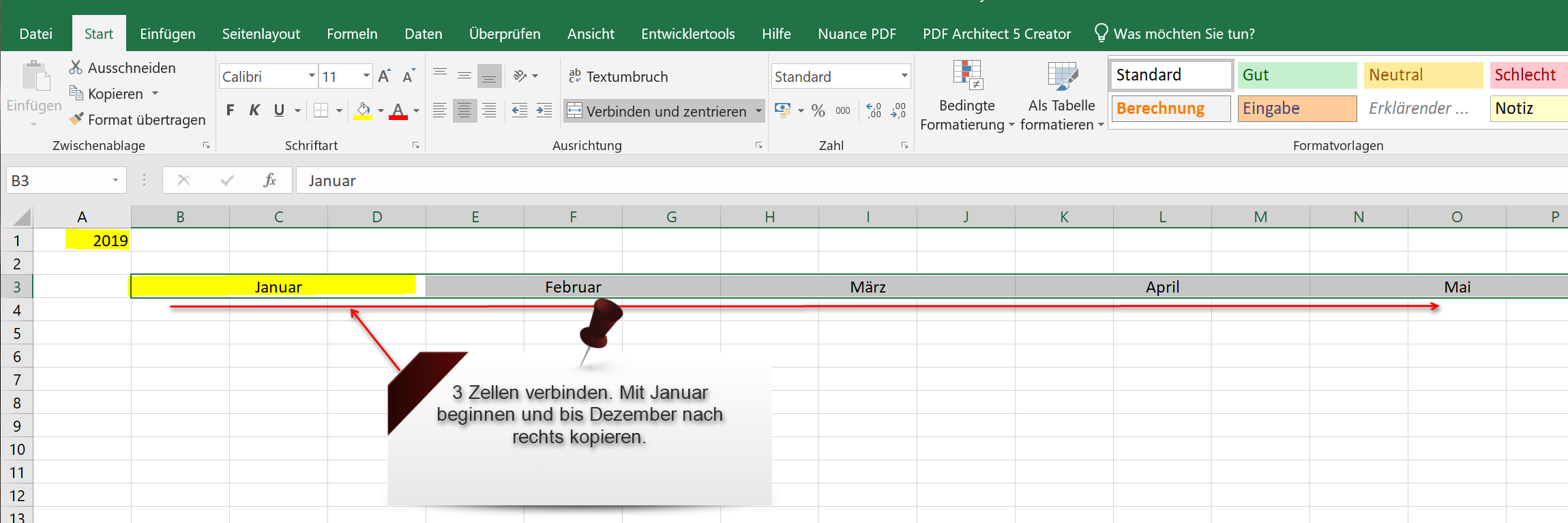
- Connect 3 cells with each other using the “Connect and center” function.
- Enter the month “January” in the first cell cluster.
- Select the cell that says “January” and copy it over to the right until December.
See fig .: (click to enlarge)
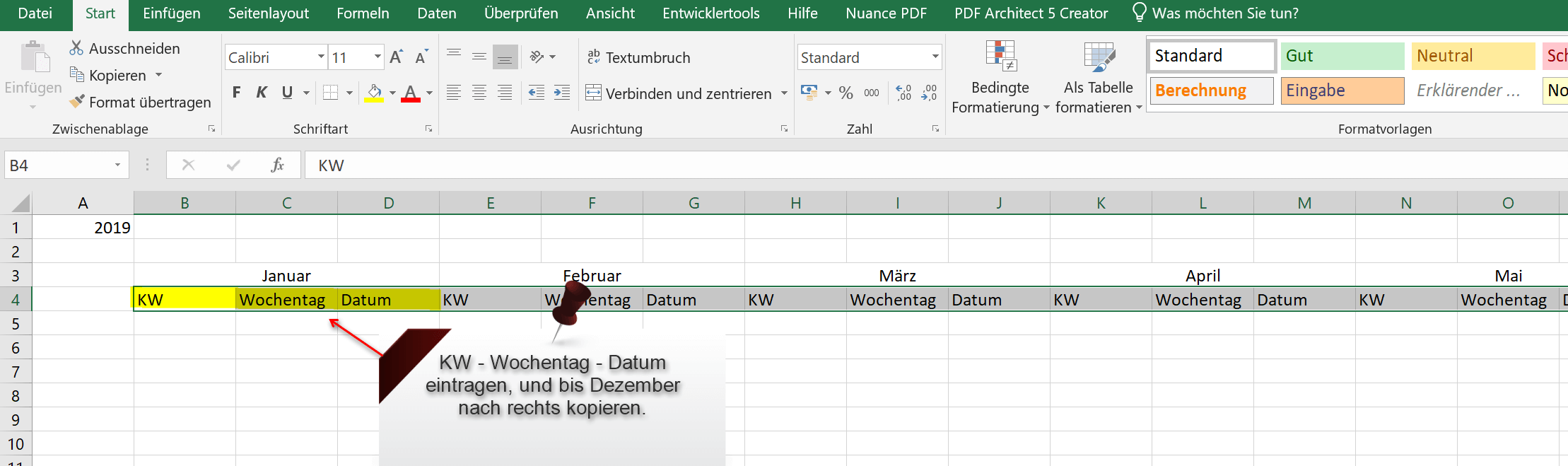
Next, enter under the line in which the months are: CW – weekday – date
You only need to do this with the first three cells under the month of January. Then select these three cells and copy them back to the right until the month of December.
See fig .: (click to enlarge)
Prepared in this way, we can start entering the first small function and format the cells accordingly.
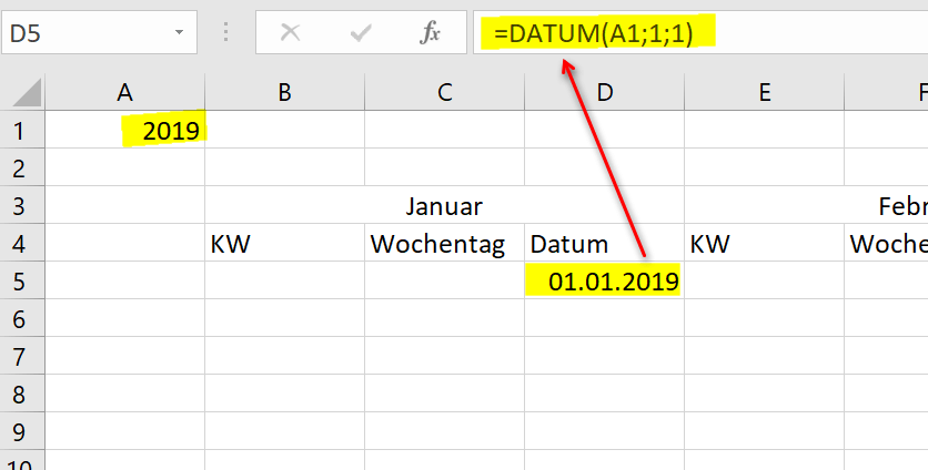
- Enter the following in the cell under “Date”: = DATE (A1; 1; 1) and confirm with Enter.
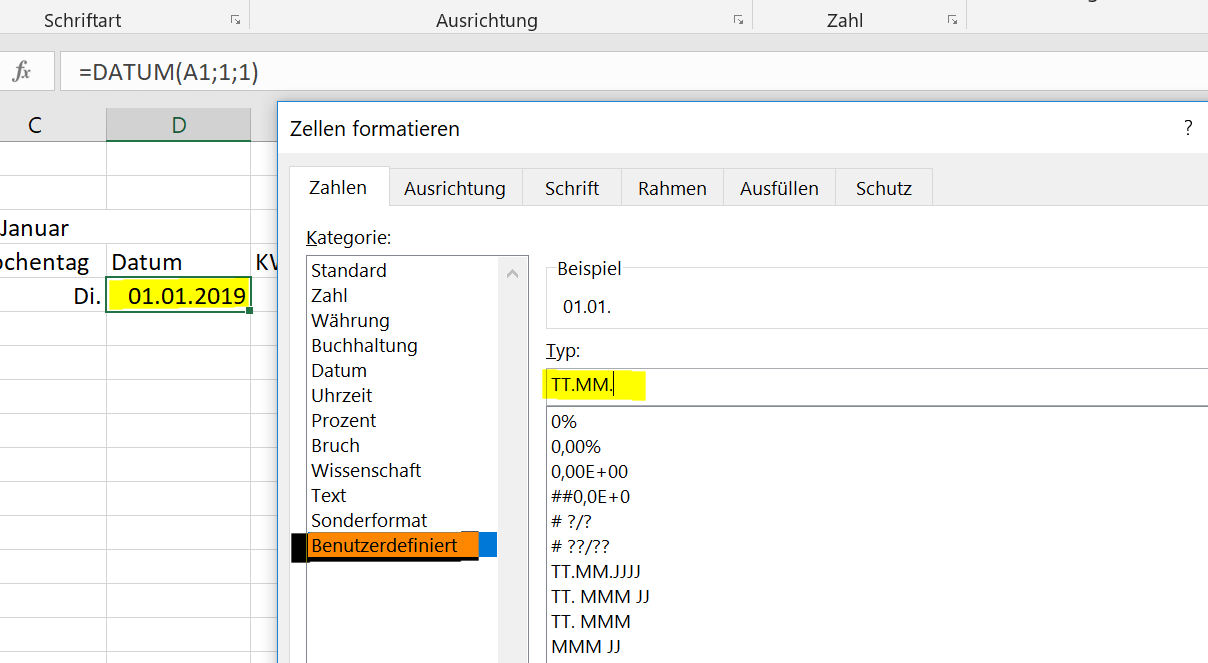
- Click in this cell in the context menu or via the menu ribbon on “Format cells”, select “Date” and “User-defined”.
- Enter DD.MM in the field for the user-defined formatting. to only display the day and month.
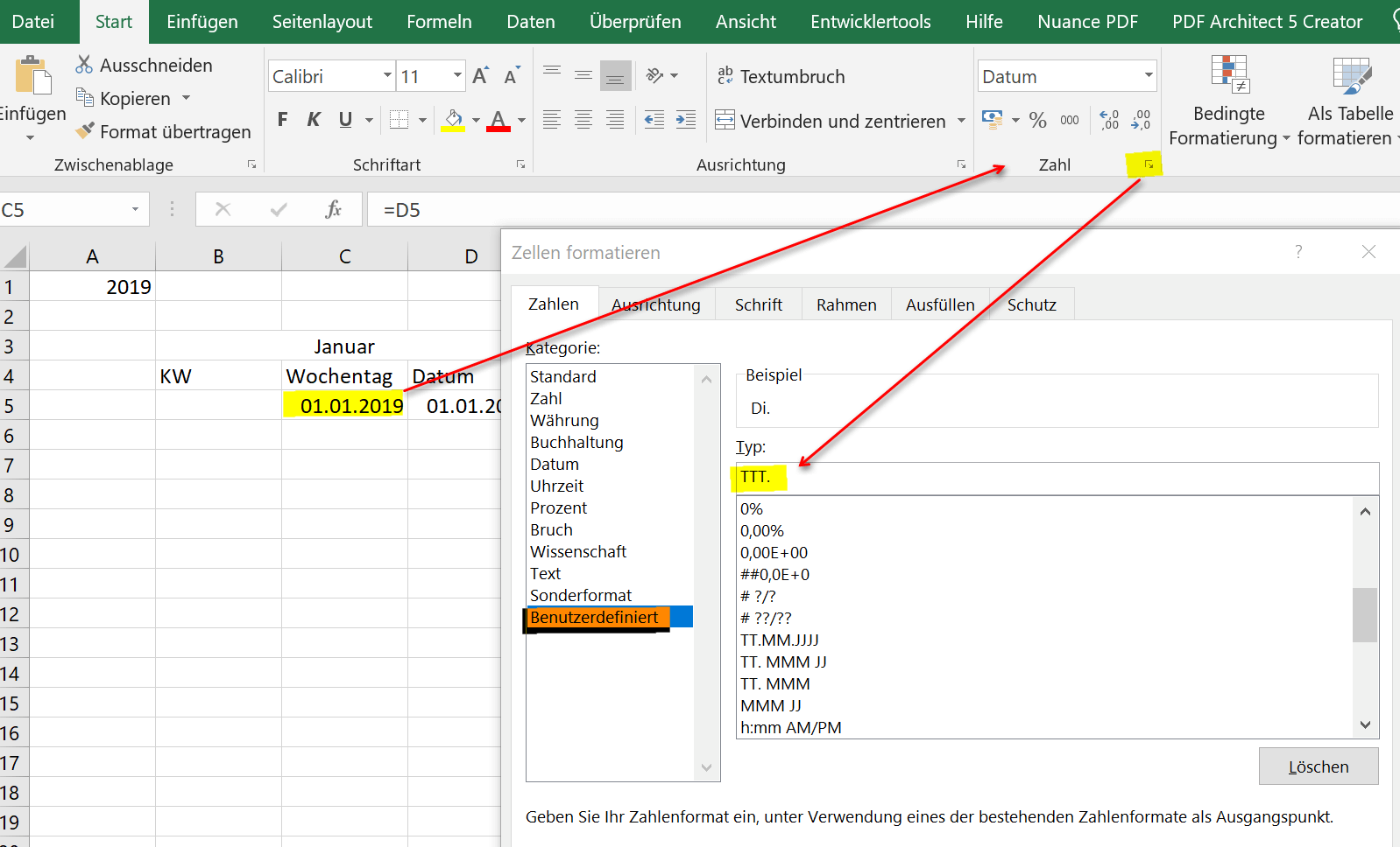
- In the cell to the left of the date created in this way, enter = D5, referring to the date cell.
- Then format this cell again as user-defined as date and enter TTT there. to only display the day of the week in abbreviated form here.
See fig .: (click to enlarge)
So that we can later create the calendar for the whole year using the Excel copy control in just a few steps, a few operations with the corresponding functions are necessary.
- Enter any year in the top line.
- Leave 2 to 3 lines below this.
- Connect 3 cells with each other using the “Connect and center” function.
- Enter the month “January” in the first cell cluster.
- Select the cell that says “January” and copy it over to the right until December.
See fig .: (click to enlarge)
Next, enter under the line in which the months are: CW – weekday – date
You only need to do this with the first three cells under the month of January. Then select these three cells and copy them back to the right until the month of December.
See fig .: (click to enlarge)
Prepared in this way, we can start entering the first small function and format the cells accordingly.
- Enter the following in the cell under “Date”: = DATE (A1; 1; 1) and confirm with Enter.
- Click in this cell in the context menu or via the menu ribbon on “Format cells”, select “Date” and “User-defined”.
- Enter DD.MM in the field for the user-defined formatting. to only display the day and month.
- In the cell to the left of the date created in this way, enter = D5, referring to the date cell.
- Then format this cell again as user-defined as date and enter TTT there. to only display the day of the week in abbreviated form here.
See fig .: (click to enlarge)
2. Enter the important functions
2. Enter the important functions
To do this, we first start with the determination of the date for the month of February:
- Enter the following in the cell under Date for February: = EDATE (D5; 1) The reference to the date cell of January is important.
- In the cell where the day of the week is, refer to the date again and format this cell as you did for January.
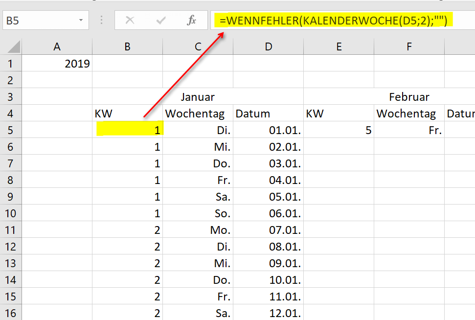
- Now mark the cell under “KW” in the month of January and enter the following there: = IF ERROR (CALENDAR WEEK (D5; 2); “”)
- Repeat the process for the cell under KW in February.
Note:
The “IF ERROR” function will later help to hide errors – which do not affect the functionality of the calendar – but which look ugly.
See fig .: (click to enlarge)


Now select the 3 cells: CW – weekday – date under the month of February, and copy this over to December on the right.
See fig .: (click to enlarge)


Next, enter the following function in the cell under 01.01: = IFERROR (IF (MONTH (D5 + 1) = MONTH (D $ 5); D5 + 1; “”); “”)
With this function, we tell Excel, in short, that a date from February does not suddenly appear in the month of January, and we also hide undesired error messages with IFERROR.
Repeat this function again in the cell under 02/01. But make sure that you also refer to the date in February and not in January.
Now you can mark the cell with 02.01, copy it down at the lower right corner of the mark until the last day of January by holding down the left mouse button. Then mark the first cell under “Day of the week” for January, and double-click left on the lower right edge of the mark.
This will automatically fill in all cells to the end.
To do this, we first start with the determination of the date for the month of February:
- Enter the following in the cell under Date for February: = EDATE (D5; 1) The reference to the date cell of January is important.
- In the cell where the day of the week is, refer to the date again and format this cell as you did for January.
- Now mark the cell under “KW” in the month of January and enter the following there: = IF ERROR (CALENDAR WEEK (D5; 2); “”)
- Repeat the process for the cell under KW in February.
Note:
The “IF ERROR” function will later help to hide errors – which do not affect the functionality of the calendar – but which look ugly.
See fig .: (click to enlarge)
Now select the 3 cells: CW – weekday – date under the month of February, and copy this over to December on the right.
See fig .: (click to enlarge)
Next, enter the following function in the cell under 01.01: = IFERROR (IF (MONTH (D5 + 1) = MONTH (D $ 5); D5 + 1; “”); “”)
With this function, we tell Excel, in short, that a date from February does not suddenly appear in the month of January, and we also hide undesired error messages with IFERROR.
Repeat this function again in the cell under 02/01. But make sure that you also refer to the date in February and not in January.
Now you can mark the cell with 02.01, copy it down at the lower right corner of the mark until the last day of January by holding down the left mouse button. Then mark the first cell under “Day of the week” for January, and double-click left on the lower right edge of the mark.
This will automatically fill in all cells to the end.
3. Highlight weekends in the calendar
3. Highlight weekends in the calendar
Now the calendar is actually ready so far that you could finish it with one copy step.
However, for our example, we want to automatically highlight the weekends beforehand and copy this function at the same time.
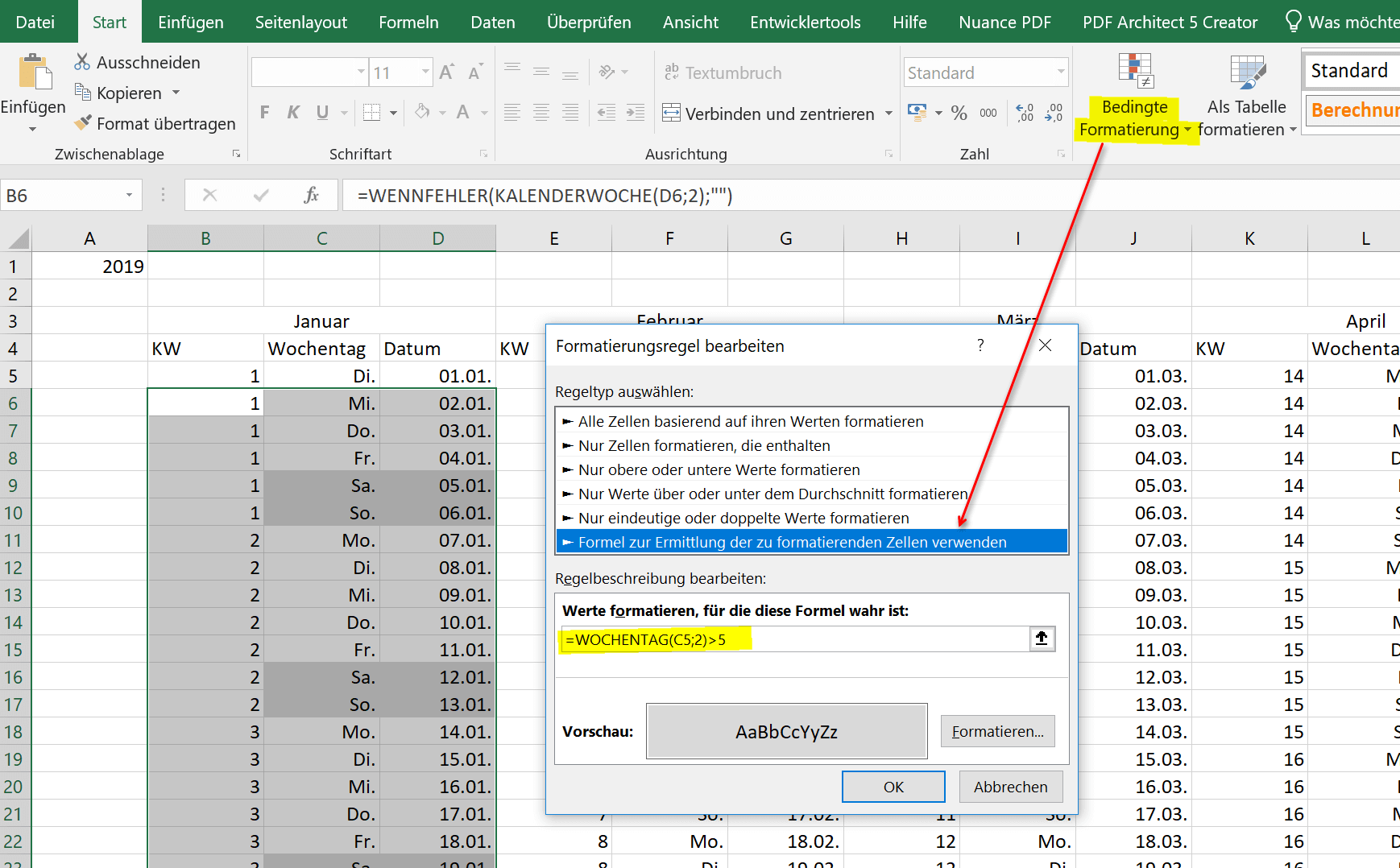
- Select the first 3 cells under the month of January and expand the selection to the end of the month.
- Then click on “Conditional Formatting” in the ribbon and select “Use formula to determine the cells to be formatted”
- Enter the following function here: = WEEKDAY (C5; 2)> 5
- Now click on “Format” and choose either a background color or a font color as desired.
- Confirm the rule with “OK”
See fig .: (click to enlarge)
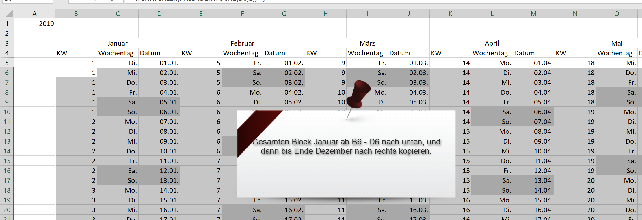
You can leave the existing marking of the cells marked as it is, and hold them on the lower right edge with the left mouse button and copy them to the right until the end of December.
And with that our calendar would already be finished (at least in the basic structure). If you now want to jump to a different year, you only need to change the year and all other values in the calendar adapt dynamically.
See fig. (Click to enlarge)
Tip:
How you can use such an annual calendar as a vacation or shift planner, for example, can also be downloaded from our offers.
Offers 2024: Word & Excel Templates


Now the calendar is actually ready so far that you could finish it with one copy step.
However, for our example, we want to automatically highlight the weekends beforehand and copy this function at the same time.
- Select the first 3 cells under the month of January and expand the selection to the end of the month.
- Then click on “Conditional Formatting” in the ribbon and select “Use formula to determine the cells to be formatted”
- Enter the following function here: = WEEKDAY (C5; 2)> 5
- Now click on “Format” and choose either a background color or a font color as desired.
- Confirm the rule with “OK”
See fig .: (click to enlarge)
You can leave the existing marking of the cells marked as it is, and hold them on the lower right edge with the left mouse button and copy them to the right until the end of December.
And with that our calendar would already be finished (at least in the basic structure). If you now want to jump to a different year, you only need to change the year and all other values in the calendar adapt dynamically.
See fig. (Click to enlarge)
Tip:
How you can use such an annual calendar as a vacation or shift planner, for example, can also be downloaded from our offers.
Offers 2024: Word & Excel Templates
Popular Posts:

Wi-Fi 7 vs. Wi-Fi 6: A quantum leap for your home network?
Wi-Fi 7 is here! Learn all about its advantages over Wi-Fi 6: extreme speed, minimal latency, and MLO. We'll explain who should upgrade now and what you can do with your ISP router. Your guide to the Wi-Fi of the future.

Microsoft 365 Copilot in practice: Your guide to the new everyday work routine
What can Microsoft 365 Copilot really do? 🤖 We'll show you in a practical way how the AI assistant revolutionizes your daily work in Word, Excel & Teams. From a blank page to a finished presentation in minutes! The ultimate practical guide for the new workday. #Copilot #Microsoft365 #AI

EU chat control: The battle between protection and privacy
The EU's chat control measures aim to scan private messages on WhatsApp and similar platforms. Critics see this as mass surveillance. Following massive resistance, including from Germany, the crucial vote in the EU Council has been postponed again. The fight for digital privacy continues.

Safe at Home: The Ultimate Guide to Your PC and Your Wi-Fi
Is your home Wi-Fi really secure? 🏠 From router passwords to phishing protection – our ultimate security guide will make life difficult for hackers. Secure your PC and home network now with our simple and easy-to-understand tips! #Cybersecurity #HomeNetwork

Integrate and use ChatGPT in Excel – is that possible?
ChatGPT is more than just a simple chatbot. Learn how it can revolutionize how you work with Excel by translating formulas, creating VBA macros, and even promising future integration with Office.

Create Out of Office Notice in Outlook
To create an Out of Office message in Microsoft Outlook - Office 365, and start relaxing on vacation
Offers 2024: Word & Excel Templates
Popular Posts:
Wi-Fi 7 vs. Wi-Fi 6: A quantum leap for your home network?
Wi-Fi 7 is here! Learn all about its advantages over Wi-Fi 6: extreme speed, minimal latency, and MLO. We'll explain who should upgrade now and what you can do with your ISP router. Your guide to the Wi-Fi of the future.
Microsoft 365 Copilot in practice: Your guide to the new everyday work routine
What can Microsoft 365 Copilot really do? 🤖 We'll show you in a practical way how the AI assistant revolutionizes your daily work in Word, Excel & Teams. From a blank page to a finished presentation in minutes! The ultimate practical guide for the new workday. #Copilot #Microsoft365 #AI
EU chat control: The battle between protection and privacy
The EU's chat control measures aim to scan private messages on WhatsApp and similar platforms. Critics see this as mass surveillance. Following massive resistance, including from Germany, the crucial vote in the EU Council has been postponed again. The fight for digital privacy continues.
Safe at Home: The Ultimate Guide to Your PC and Your Wi-Fi
Is your home Wi-Fi really secure? 🏠 From router passwords to phishing protection – our ultimate security guide will make life difficult for hackers. Secure your PC and home network now with our simple and easy-to-understand tips! #Cybersecurity #HomeNetwork
Integrate and use ChatGPT in Excel – is that possible?
ChatGPT is more than just a simple chatbot. Learn how it can revolutionize how you work with Excel by translating formulas, creating VBA macros, and even promising future integration with Office.
Create Out of Office Notice in Outlook
To create an Out of Office message in Microsoft Outlook - Office 365, and start relaxing on vacation
Offers 2024: Word & Excel Templates