How to create a dynamic table in Excel
A simple table is quickly created in Excel, and using a few filters to sort the data is not a problem for most.
However, the function of having Excel generate a dynamic table from existing data is rarely used, as many do not really know what is possible with this option and what advantages it offers.
In this article, we would like to describe how you can turn static tables into dynamic ones, which possibilities and advantages a dynamic table offers, and also how you can convert them back into a normal static table.
1. Creating a dynamic table
1. Creating a dynamic table
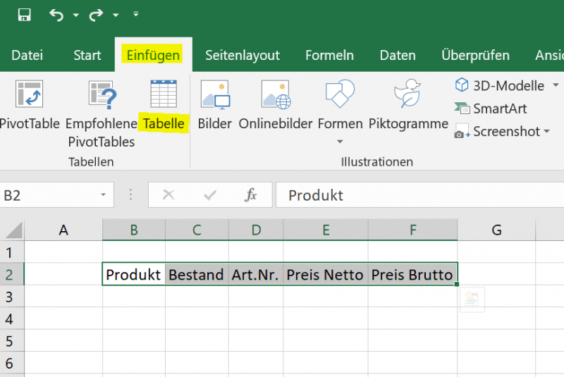
Creating a dynamic spreadsheet in Excel is actually very easy. You can do this by simply clicking in any cell and then on the “Insert” tab on “Table”.
Or you have already created a static table with headings and want to convert it to a dynamic table. To do this, simply mark the table area that is to be converted and then go to “Insert” and “Table”.
See fig.(click to enlarge)
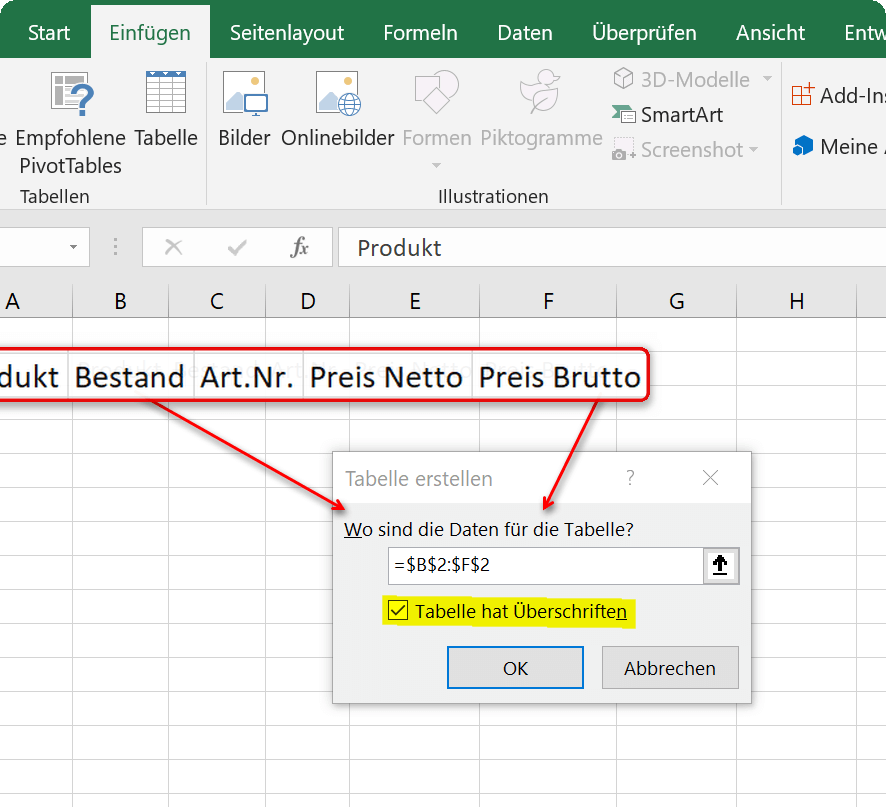

When you insert the table, you will also be asked whether the table has headings, and you may have to confirm this with a tick. If you already have headings, as in our example, you should also check the box, otherwise Excel will insert an additional line with column headings above your headings that is not required.
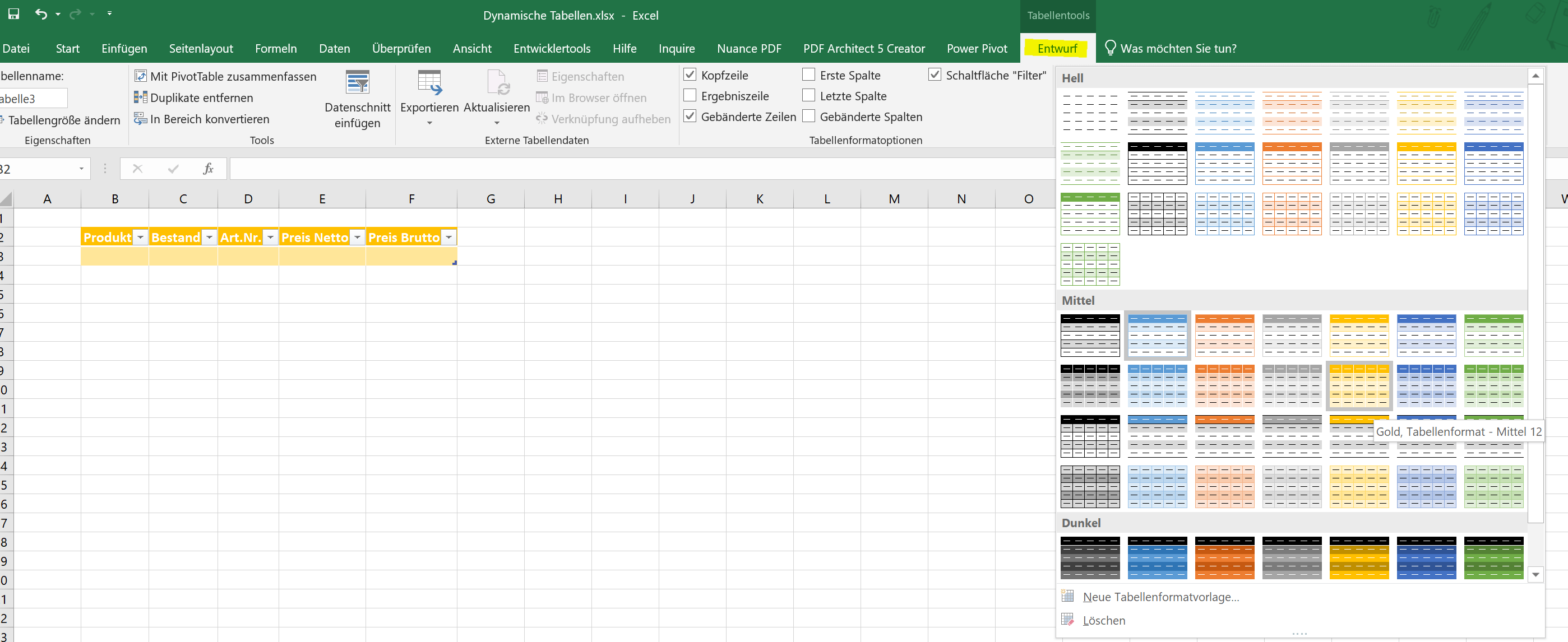
You can now change the dynamic table created in this way from one of the predefined color patterns in the layout, or you can also create your own color pattern. To do this, simply click in the table and then in the “Table Tools” – “Design” tab on the table format templates.
See fig.(click to enlarge)
Creating a dynamic spreadsheet in Excel is actually very easy. You can do this by simply clicking in any cell and then on the “Insert” tab on “Table”.
Or you have already created a static table with headings and want to convert it to a dynamic table. To do this, simply mark the table area that is to be converted and then go to “Insert” and “Table”.
See fig.(click to enlarge)
When you insert the table, you will also be asked whether the table has headings, and you may have to confirm this with a tick. If you already have headings, as in our example, you should also check the box, otherwise Excel will insert an additional line with column headings above your headings that is not required.
You can now change the dynamic table created in this way from one of the predefined color patterns in the layout, or you can also create your own color pattern. To do this, simply click in the table and then in the “Table Tools” – “Design” tab on the table format templates.
See fig.(click to enlarge)
2. Calculating with dynamic tables
2. Calculating with dynamic tables
With the newly created dynamic table, it is now also relatively easy to calculate.
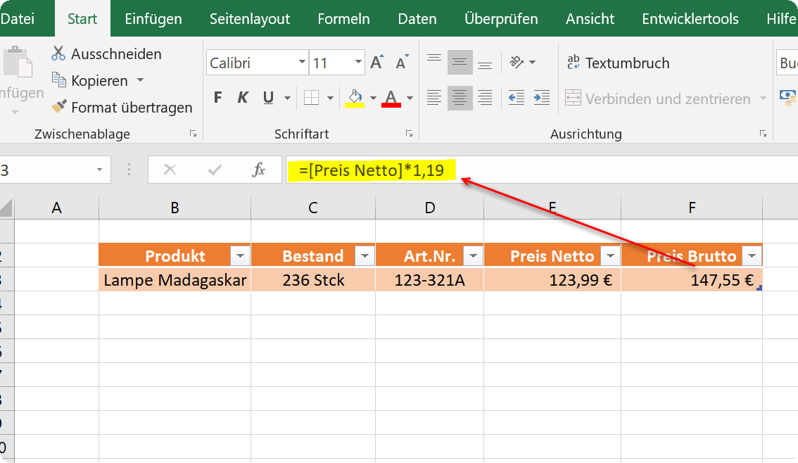
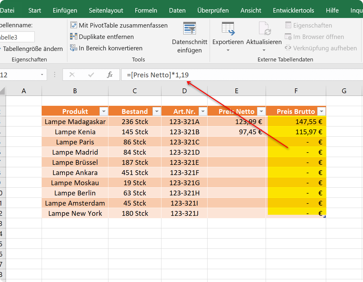
In our example, we simply created different products and calculated the gross price. To do this, we click in the cell in which the result should be and start with an “=”, as with any formula. Then we click in the first cell with the net price and multiply this value by 1.19 to calculate the 19% mark-up.
What is immediately noticeable in the formula bar is that the cell is not specified as the reference point, as in a static table, but the column heading. In this way, the formula in each new row for this area is inherited within the dynamic table, so that it does not have to be re-entered.
Of course, a table created in this way offers a number of other options and possibilities, which you can find in the “Design” tab under “Table tools”.
See fig.(click to enlarge)
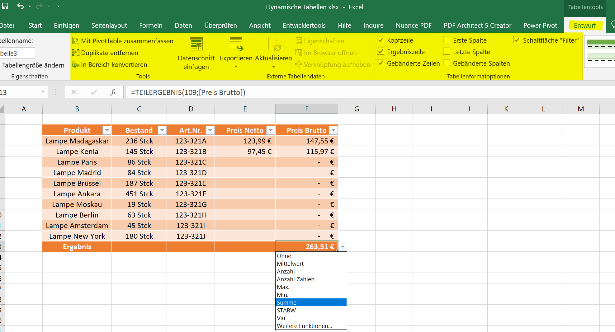
A notice:
You can either extend the table by pressing the TAB key once in the last cell of the last row of the table, or you can simply drag down the lower right edge with the left mouse button.
With the newly created dynamic table, it is now also relatively easy to calculate.
In our example, we simply created different products and calculated the gross price. To do this, we click in the cell in which the result should be and start with an “=”, as with any formula. Then we click in the first cell with the net price and multiply this value by 1.19 to calculate the 19% mark-up.
What is immediately noticeable in the formula bar is that the cell is not specified as the reference point, as in a static table, but the column heading. In this way, the formula in each new row for this area is inherited within the dynamic table, so that it does not have to be re-entered.
Of course, a table created in this way offers a number of other options and possibilities, which you can find in the “Design” tab under “Table tools”.
See fig.(click to enlarge)
A notice:
You can either extend the table by pressing the TAB key once in the last cell of the last row of the table, or you can simply drag down the lower right edge with the left mouse button.
3. Converting a dynamic table to a convertible range
3. Converting a dynamic table to a convertible range
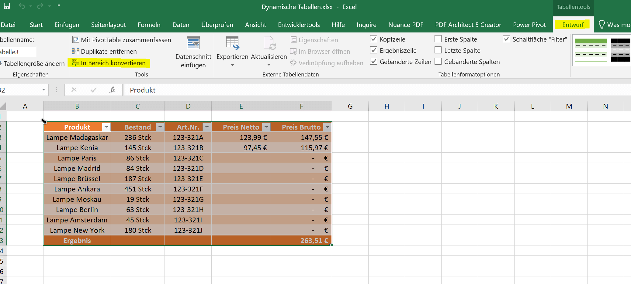
If at some point you want to convert the table back into a static table, you can do this again via the “Design” tab under “Table tools”. Simply select the entire dynamic table and then click “Convert to range”. You then only have to confirm a security query, and the dynamic table is resolved with all functions.
All previously created calculations are of course retained.
See fig.(click to enlarge)
Popular Posts:

How AI fuels cyberattacks – and how it protects us from them
Cybercriminals are using AI for deepfakes and automated attacks. Defenses are also relying on AI: through behavioral analysis (UEBA) and automated responses (SOAR). Learn how this arms race works and how modern security strategies can protect your business.

Information overload: Protection & tips against digital stress
Constantly online, overwhelmed by news, emails & social media? Digital information overload leads to stress and concentration problems. Learn the best strategies and practical tips to effectively protect yourself, manage the chaos, and regain your focus.

Put an end to password chaos: Why a password manager is important
Passwords are constantly being stolen through data leaks. A password manager is your digital vault. It creates and stores strong, unique passwords for every service. This effectively protects you against identity theft through "credential stuffing".

Stop procrastinating: How distraction blockers can help you regain focus
Constant digital distractions kill your productivity. Distraction blockers like Forest or Freedom help you regain focus. They specifically block distractions on your PC and mobile phone and use techniques like the Pomodoro Technique. This helps you stop procrastinating.
Wer ist wo? Microsoft Teams schafft Klarheit im Hybrid-Büro
Die neue Arbeitsstandort-Funktion in Microsoft Teams zeigt, wer im Büro oder remote arbeitet. Verbessern Sie Ihre Meeting-Planung in Outlook und die Team-Koordination. Wir erklären die Vorteile, die Admin-Steuerung und die tiefe Anbindung an Microsoft Viva.

Excel Tutorial: How to quickly and safely remove duplicates
Duplicate entries in your Excel lists? This distorts your data. Our tutorial shows you, using a practical example, how to clean up your data in seconds with the "Remove Duplicates" function – whether you want to delete identical rows or just values in a column.
Offers 2024: Word & Excel Templates


Popular Posts:
How AI fuels cyberattacks – and how it protects us from them
Cybercriminals are using AI for deepfakes and automated attacks. Defenses are also relying on AI: through behavioral analysis (UEBA) and automated responses (SOAR). Learn how this arms race works and how modern security strategies can protect your business.
Information overload: Protection & tips against digital stress
Constantly online, overwhelmed by news, emails & social media? Digital information overload leads to stress and concentration problems. Learn the best strategies and practical tips to effectively protect yourself, manage the chaos, and regain your focus.
Put an end to password chaos: Why a password manager is important
Passwords are constantly being stolen through data leaks. A password manager is your digital vault. It creates and stores strong, unique passwords for every service. This effectively protects you against identity theft through "credential stuffing".
Stop procrastinating: How distraction blockers can help you regain focus
Constant digital distractions kill your productivity. Distraction blockers like Forest or Freedom help you regain focus. They specifically block distractions on your PC and mobile phone and use techniques like the Pomodoro Technique. This helps you stop procrastinating.
Wer ist wo? Microsoft Teams schafft Klarheit im Hybrid-Büro
Die neue Arbeitsstandort-Funktion in Microsoft Teams zeigt, wer im Büro oder remote arbeitet. Verbessern Sie Ihre Meeting-Planung in Outlook und die Team-Koordination. Wir erklären die Vorteile, die Admin-Steuerung und die tiefe Anbindung an Microsoft Viva.
Excel Tutorial: How to quickly and safely remove duplicates
Duplicate entries in your Excel lists? This distorts your data. Our tutorial shows you, using a practical example, how to clean up your data in seconds with the "Remove Duplicates" function – whether you want to delete identical rows or just values in a column.
Offers 2024: Word & Excel Templates