The Sreference and the Wreference in Excel
If you have created a table with many records in Excel, you may eventually come to a point where certain records should be automatically retrieved from this table and pasted into another table for a better overview.
So what do you do?
Of course you have the possibility to create one or more stand-alone tables with the Pivot function, and of course have a great variety of filter options at the same time.
But sometimes it does not work the way you had imagined.
And this is exactly where the S-reference and W-reference functions come into play.
How these two variants work and how to use them I would like to shed some light on in this article.
1. Definition S-reference and W-reference
1. Definition S-reference and W-reference
In general we first clarify the definition of the S-reference and W-reference.
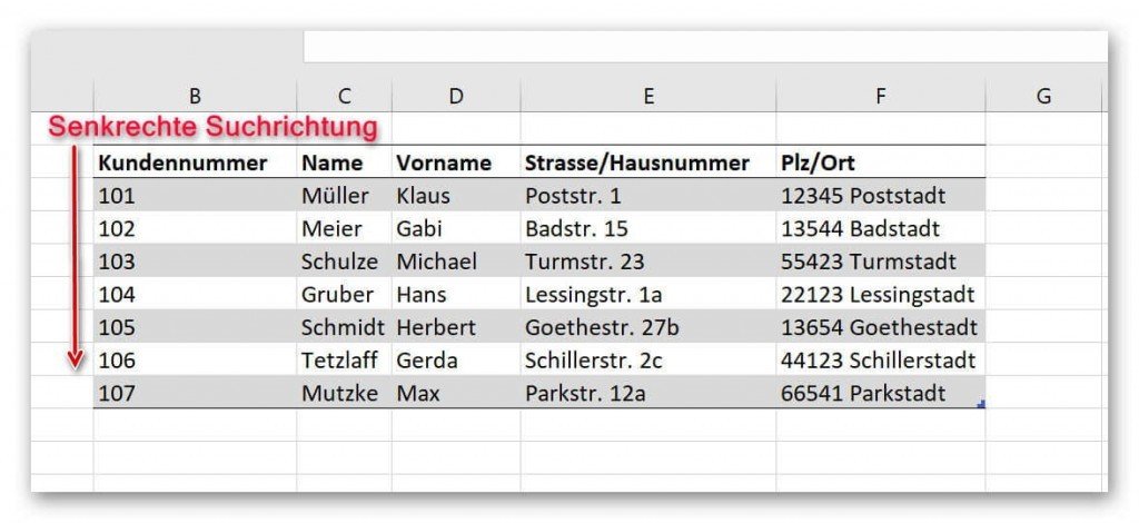
The S-reference:
The “S” stands for “vertical” and describes the search direction in which Excel searches for a specific term.
What does this mean in columns for a term is searched, and if this is found is searched in the appropriate line to determine the coordinate.
see picture: (click to enlarge)
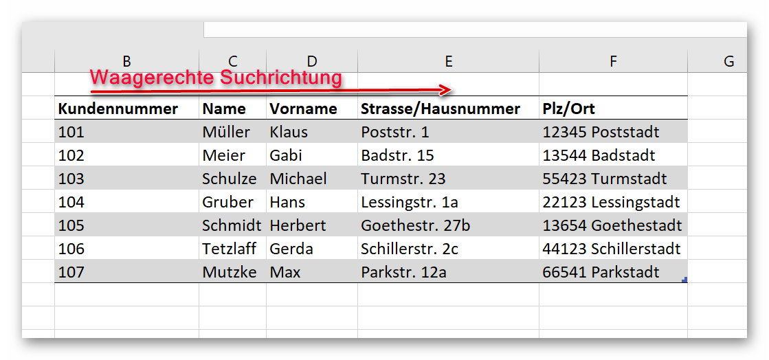
The W reference:
The “W” stands for “horizontal” and also describes the search direction in which Excel searches for a specific term.
Only here is not determined first in columns but in lines for a specific term to determine the coordinate.
see picture: (click to enlarge)

In general we first clarify the definition of the S-reference and W-reference.
The S-reference:
The “S” stands for “vertical” and describes the search direction in which Excel searches for a specific term.
What does this mean in columns for a term is searched, and if this is found is searched in the appropriate line to determine the coordinate.
see picture: (click to enlarge)

The W reference:
The “W” stands for “horizontal” and also describes the search direction in which Excel searches for a specific term.
Only here is not determined first in columns but in lines for a specific term to determine the coordinate.
see picture: (click to enlarge)
2. Procedure S-reference
2. Procedure S-reference
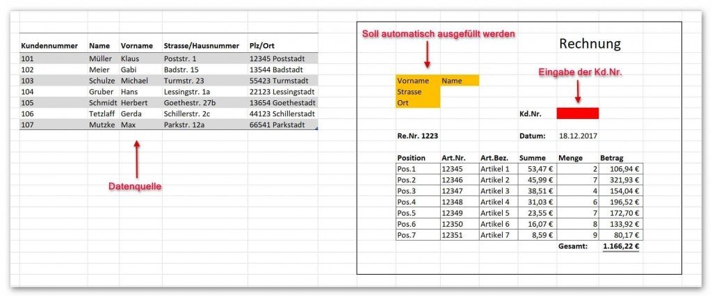
In order to make the whole thing a bit more plastic let’s assume that we want to build a bill template in Excel, but do not want to have to enter all the recipient data (name, street, city) every time.
Then we should begin by creating a suitable table of customer master data that will later serve as the data source for our S reference. Next, of course, we need the destination (our invoice template).
In the invoice, the recipient address is to be filled in automatically after entering the customer number.
see picture: (click to enlarge)
For the automated filling of the receiver head to work, we now need to build several S references that all use the same source but need different coordinates to output the correct data set.
The first entry: first name
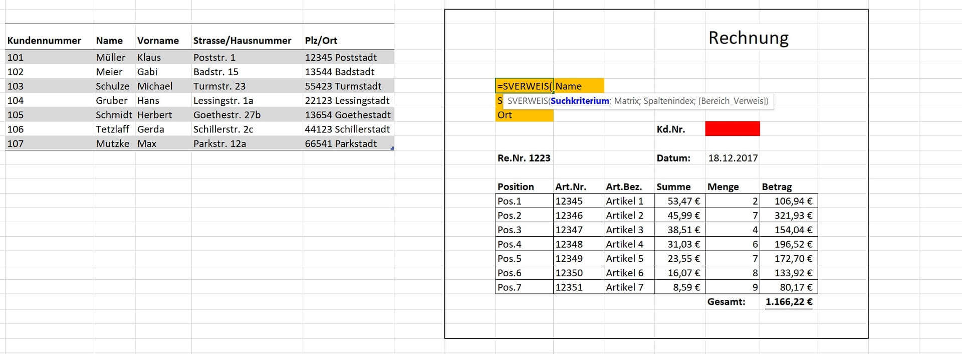
We click in the cell “First name” and start by entering the formula as follows:
= LOOKUP (
- After this input, Excel will already tell us which information is needed first. This is the search criteria.
- Here we have to click on the cell in which we will enter our customer number later.
What does Excel do after exactly what is entered there will look in the data source.
see picture: (click to enlarge)
Next, Excel asks for the matrix which is nothing but the table area in which to search for the search criterion (our customer number).
In our example, we can easily mark the entire table with our customer master data.
see picture: (click to enlarge)
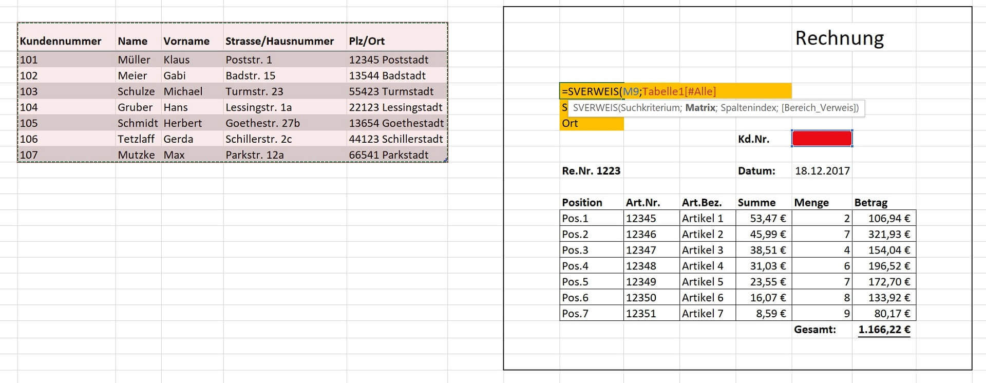
Be sure to remember all the arguments in the formula are each with a semicolon; to separate.
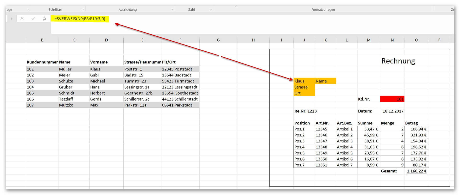
The next step asks for the column index.
Here is simply counted. And in the wievielt column of the previously marked table (not the entire worksheet!) Is to be searched for the entry in the field “first name” should.
In our example, it is the third column (in which the first names are). Thus, we simply enter a 3 here.
The last part of our S-reference is not entirely unimportant, because it asks for true = 1 or false = 0.
This is a bit confusing at first, but ultimately means nothing else if Excel should search for exactly the search criterion (as it was entered), or whether it may be similar.
For our example, of course, we are looking for exactly the name entered, and not one of the similar.
So we enter a “0”.
Our finished S-reference for the first field “first name” should look like this.
see picture: (click to enlarge)
In order to make the whole thing a bit more plastic let’s assume that we want to build a bill template in Excel, but do not want to have to enter all the recipient data (name, street, city) every time.
Then we should begin by creating a suitable table of customer master data that will later serve as the data source for our S reference. Next, of course, we need the destination (our invoice template).
In the invoice, the recipient address is to be filled in automatically after entering the customer number.
see picture:

For the automated filling of the receiver head to work, we now need to build several S references that all use the same source but need different coordinates to output the correct data set.
The first entry: first name
We click in the cell “First name” and start by entering the formula as follows:
= LOOKUP (
- After this input, Excel will already tell us which information is needed first. This is the search criteria.
- Here we have to click on the cell in which we will enter our customer number later.
What does Excel do after exactly what is entered there will look in the data source.
see picture:

Next, Excel asks for the matrix which is nothing but the table area in which to search for the search criterion (our customer number).
In our example, we can easily mark the entire table with our customer master data.
see picture:

Be sure to remember all the arguments in the formula are each with a semicolon; to separate.
The next step asks for the column index.
Here is simply counted. And in the wievielt column of the previously marked table (not the entire worksheet!) Is to be searched for the entry in the field “first name” should.
In our example, it is the third column (in which the first names are). Thus, we simply enter a 3 here.
The last part of our S-reference is not entirely unimportant, because it asks for true = 1 or false = 0.
This is a bit confusing at first, but ultimately means nothing else if Excel should search for exactly the search criterion (as it was entered), or whether it may be similar.
For our example, of course, we are looking for exactly the name entered, and not one of the similar.
So we enter a “0”.
Our finished S-reference for the first field “first name” should look like this.
see picture:
3. Procedure W-reference
3. Procedure W-reference
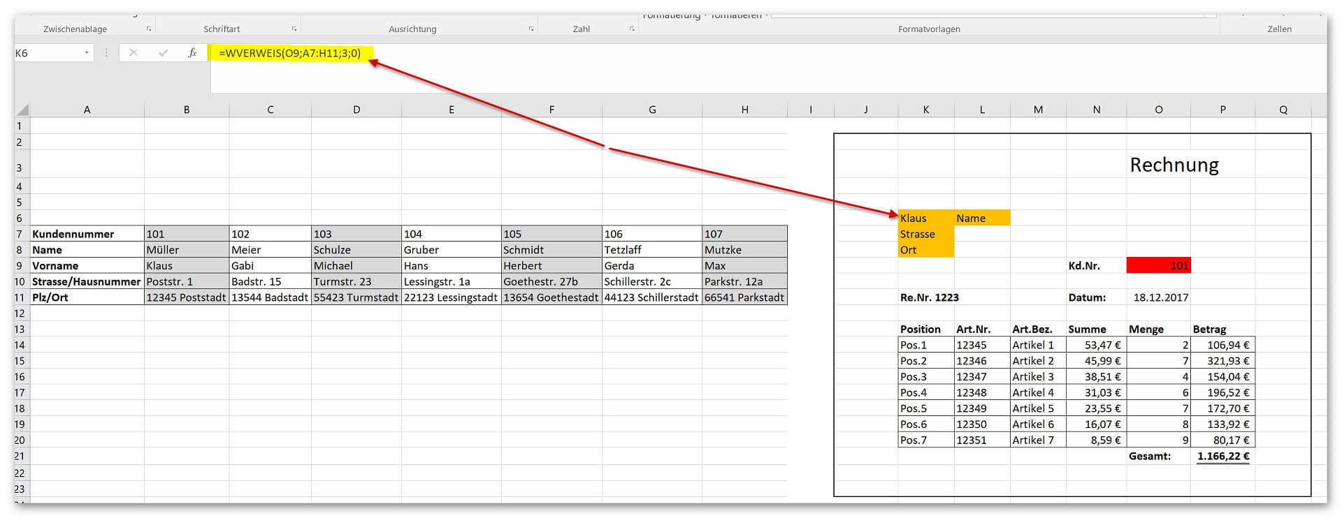
The W reference is relatively similar to the S reference.
The main difference lies in the search direction.
It is not searched vertically but horizontally. To stay with our calculation example, I simply transposed the table with the data source (lines and columns reversed) to represent the W reference.
The function with which we come to our “first name” in the bill is therefore:
= HLOOKUP (
Then again specify the cell with the search criterion (the one with the customer number)
next the matrix area (the whole table with the master data)
and now, instead of a column index, just get a row index.
Again, we just count by again. And in which line should be searched for the first name.
This is the third line in our example. So we enter the 3 at the line index.
And finally, we enter the “0” for “False” to search for an exact match.
Our complete function should look like this.
see picture: (click to enlarge)
Both the S-reference and the W-reference can be used in such a variety of ways, and lead depending on the starting position of the data source to one and the same result.
Of course, you can extend the whole range of functions considerably, and nest them with other functions as well (for example with an if-then function), but already in the basic version, some of the work can be done well with these rather simple functions.
The W reference is relatively similar to the S reference.
The main difference lies in the search direction.
It is not searched vertically but horizontally. To stay with our calculation example, I simply transposed the table with the data source (lines and columns reversed) to represent the W reference.
The function with which we come to our “first name” in the bill is therefore:
= HLOOKUP (
Then again specify the cell with the search criterion (the one with the customer number)
next the matrix area (the whole table with the master data)
and now, instead of a column index, just get a row index.
Again, we just count by again. And in which line should be searched for the first name.
This is the third line in our example. So we enter the 3 at the line index.
And finally, we enter the “0” for “False” to search for an exact match.
Our complete function should look like this.
see picture: (click to enlarge)
Der W-Verweis ist dem S-Verweis relativ gleich.
Der Hauptunterschied liegt hierbei in der Suchrichtung. Es wird hier also nicht senkrecht sondern waagerecht gesucht. Um bei unserem Rechnungsbeispiel zu bleiben, habe ich die Tabelle mit der Datenquelle einfach mal transponiert (Zeilen und Spalten vertauscht) um den W-Verweis darzustellen.
Die Funktion mit der wir zu unserem “Vornamen” in der Rechnung kommen lautet demnach: =WVERWEIS(
Dann erneut die Zelle mit dem Suchkriterium festlegen (Die mit der Kundennummer) als nächstes den Matrixbereich (Die gesamte Tabelle mit den Stammdaten) und nun kommt statt einem Spaltenindex einfach ein Zeilenindex.
Auch hier zählen wir einfach wieder durch. Und zwar in welcher Zeile soll nach dem Vornamen gesucht werden.
Dies ist in unserem Beispiel die dritte Zeile. Also geben wir beim Zeilenindex die 3 ein. Und zum Schluss geben wir noch die “0” für “Falsch” ein, damit nach einer genauen Übereinstimmung gesucht wird.
Unsere komplette Funktion sollte dann wie folgt aussehen.
siehe Abb.:

Both the S-reference and the W-reference can be used in such a variety of ways, and lead depending on the starting position of the data source to one and the same result.
Of course, you can extend the whole range of functions considerably, and nest them with other functions as well (for example with an if-then function), but already in the basic version, some of the work can be done well with these rather simple functions.
Popular Posts:

Ad-free home network: Install Pi-hole on Windows
Say goodbye to ads on smart TVs and in apps: Pi-hole software turns your Windows laptop into a network filter. This article explains step-by-step how to install it via Docker and configure the necessary DNS settings in your FRITZ!Box.

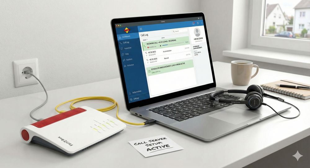
How to tune your FRITZ!Box into a professional call server
A professional telephone system can be built using a FRITZ!Box and a laptop. This article shows step by step how to use the free software "Phoner" to schedule announcements and record calls – including important legal information (§ 201 StGB).

Why to-do lists are a waste of time
Do you feel unproductive at the end of the day, even though you've worked hard? Your to-do list is to blame. It tempts you to focus on easy tasks and ignores your limited time. This article explains why lists are "self-deception" and why professionals use a calendar instead.

Smartphone Wi-Fi security: Public hotspots vs. home network
Is smartphone Wi-Fi a security risk? This article analyzes in detail threats such as evil twin attacks and explains protective measures for when you're on the go. We also clarify why home Wi-Fi is usually secure and how you can effectively separate your smart home from sensitive data using a guest network.

Warum dein Excel-Kurs Zeitverschwendung ist – was du wirklich lernen solltest!
Hand aufs Herz: Wann hast du zuletzt eine komplexe Excel-Formel ohne Googeln getippt? Eben. KI schreibt heute den Code für dich. Erfahre, warum klassische Excel-Trainings veraltet sind und welche 3 modernen Skills deinen Marktwert im Büro jetzt massiv steigern.

Cybersicherheit: Die 3 größten Fehler, die 90% aller Mitarbeiter machen
Hacker brauchen keine Codes, sie brauchen nur einen unaufmerksamen Mitarbeiter. Von Passwort-Recycling bis zum gefährlichen Klick: Wir zeigen die drei häufigsten Fehler im Büroalltag und geben praktische Tipps, wie Sie zur menschlichen Firewall werden.
Offers 2024: Word & Excel Templates


Popular Posts:
Ad-free home network: Install Pi-hole on Windows
Say goodbye to ads on smart TVs and in apps: Pi-hole software turns your Windows laptop into a network filter. This article explains step-by-step how to install it via Docker and configure the necessary DNS settings in your FRITZ!Box.
How to tune your FRITZ!Box into a professional call server
A professional telephone system can be built using a FRITZ!Box and a laptop. This article shows step by step how to use the free software "Phoner" to schedule announcements and record calls – including important legal information (§ 201 StGB).
Why to-do lists are a waste of time
Do you feel unproductive at the end of the day, even though you've worked hard? Your to-do list is to blame. It tempts you to focus on easy tasks and ignores your limited time. This article explains why lists are "self-deception" and why professionals use a calendar instead.
Smartphone Wi-Fi security: Public hotspots vs. home network
Is smartphone Wi-Fi a security risk? This article analyzes in detail threats such as evil twin attacks and explains protective measures for when you're on the go. We also clarify why home Wi-Fi is usually secure and how you can effectively separate your smart home from sensitive data using a guest network.
Warum dein Excel-Kurs Zeitverschwendung ist – was du wirklich lernen solltest!
Hand aufs Herz: Wann hast du zuletzt eine komplexe Excel-Formel ohne Googeln getippt? Eben. KI schreibt heute den Code für dich. Erfahre, warum klassische Excel-Trainings veraltet sind und welche 3 modernen Skills deinen Marktwert im Büro jetzt massiv steigern.
Cybersicherheit: Die 3 größten Fehler, die 90% aller Mitarbeiter machen
Hacker brauchen keine Codes, sie brauchen nur einen unaufmerksamen Mitarbeiter. Von Passwort-Recycling bis zum gefährlichen Klick: Wir zeigen die drei häufigsten Fehler im Büroalltag und geben praktische Tipps, wie Sie zur menschlichen Firewall werden.
Offers 2024: Word & Excel Templates