Custom Formatting Excel – Number Format Codes Excel
Cell formatting is one of the most important core functions in Excel, with which we can make the background behind the pure numbers visible. In addition to the usual number formatting such as percent (%), currency (€/$), time (12:30), fractions (1/4) that most people know and have already used in everyday work, there is a whole range more of user-defined cell formatting and number formats that are already prepared in Excel for selection.

But often even these are not enough to display numerical values as required. For example, if you want to display a number of pallets or crates / cartons or other things in Excel in such a way that these numerical values can also be used for calculations, you will of course not find this in the existing user-defined number formatting.
The same applies to the automatic display of negative values (-1000) in a specific color. But that’s exactly why Excel offers the possibility to adapt the cell formatting to your own needs. In our little tutorial we would like to explain what the character sets (# | [] | E+ | % | ?) are all about and how you can use them. You can also find more information about cell formatting in Excel in our tutorial on conditional formatting in Excel.
Custom Formatting Excel – Number Format Codes Excel
Cell formatting is one of the most important core functions in Excel, with which we can make the background behind the pure numbers visible. In addition to the usual number formatting such as percent (%), currency (€/$), time (12:30), fractions (1/4) that most people know and have already used in everyday work, there is a whole range more of user-defined cell formatting and number formats that are already prepared in Excel for selection.
But often even these are not enough to display numerical values as required. For example, if you want to display a number of pallets or crates / cartons or other things in Excel in such a way that these numerical values can also be used for calculations, you will of course not find this in the existing user-defined number formatting.
The same applies to the automatic display of negative values (-1000) in a specific color. But that’s exactly why Excel offers the possibility to adapt the cell formatting to your own needs. In our little tutorial we would like to explain what the character sets (# | [] | E+ | % | ?) are all about and how you can use them. You can also find more information about cell formatting in Excel in our tutorial on conditional formatting in Excel.
What do the characters in custom formatting mean?
Custom formatting in Excel is accessed from the Home tab, then the Number menu section. There is usually the value “Standard” which contains a number of predefined number formattings that are used most frequently via a drop-down menu. The last item there is “further number formats” which takes you to the cell formatting area. Here you can set a lot more such as fonts, frames, color highlights.
Via “Additional number formats” you get to a dialog window in which “User-defined” is the last item. In the list that is then available for selection, it can be quite confusing what all the rhombuses, square brackets, question marks and semicolons mean and how they can be used.
see fig. (click to enlarge)
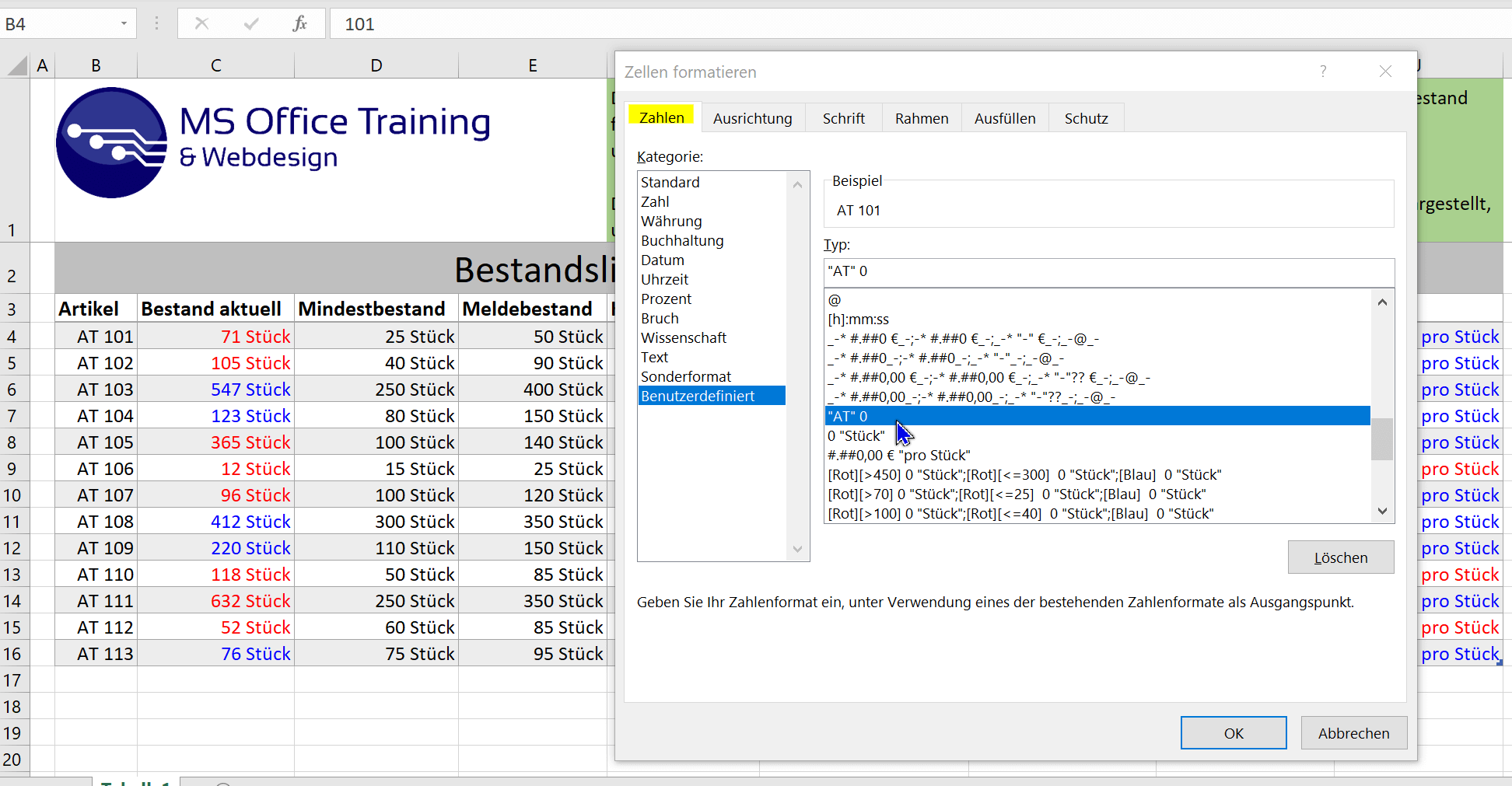

Don’t get confused at this point, because the symbols shown are nothing more than placeholders for specific applications. You can accept it, but you don’t have to. You can also build your own use case from it, or adapt predefined formatting that is in the list (almost) arbitrarily. Below is a table of symbols and what they stand for:
| Number format code | meaning |
|---|---|
| # | Placeholder for numbers that can be used to limit the number of zeros within a number to the significant number |
| “” | For inserting text in combination with numbers (e.g. 100 “palettes”) |
| [] | For defining text or numbers in a specific color (e.g. [red], [green], [blue]) |
| = | Condition for a numerical value that fulfills a condition (e.g. > than 1,000) |
| <> | Less than and Greater than… (Can be combined with “=” e.g. >=1000 |
| €, $, £, ¥ | Currency formatting determines where the currency symbol appears, and it also determines the style and position of the thousands separator |
| E+, E-, e+, e- | Scientific format for displaying the exponent. Number of zeros or “#” indicates the number of digits in the exponent. “E-” or “e-” (negative exponents) displays a minus sign, and “E+” and “+” (positive exponents) displays a plus sign |
| yy, dd, mm, ss, hh | Formatting of time-based numerical values. This can be years, months, days, hours, minutes or seconds, which can be output in different ways (depending on the number of codes used). (Ex. Jan 14, 2022 = dd:mmmm:yyy or Jan 14, 2022 = dd:mm:yy) |
| ? | Used to display fractions (e.g. 5.25 = 5 1/4 = #?/?). The hash indicates the place for the whole number, and with ?/? specifies that the decimal places should be displayed as a fraction |
What do the characters in custom formatting mean?
Custom formatting in Excel is accessed from the Home tab, then the Number menu section. There is usually the value “Standard” which contains a number of predefined number formattings that are used most frequently via a drop-down menu. The last item there is “further number formats” which takes you to the cell formatting area. Here you can set a lot more such as fonts, frames, color highlights.
Via “Additional number formats” you get to a dialog window in which “User-defined” is the last item. In the list that is then available for selection, it can be quite confusing what all the rhombuses, square brackets, question marks and semicolons mean and how they can be used.
see fig. (click to enlarge)
Don’t get confused at this point, because the symbols shown are nothing more than placeholders for specific applications. You can accept it, but you don’t have to. You can also build your own use case from it, or adapt predefined formatting that is in the list (almost) arbitrarily. Below is a table of symbols and what they stand for:
| Number format code | meaning |
|---|---|
| # | Placeholder for numbers that can be used to limit the number of zeros within a number to the significant number |
| “” | For inserting text in combination with numbers (e.g. 100 “palettes”) |
| [] | For defining text or numbers in a specific color (e.g. [red], [green], [blue]) |
| = | Condition for a numerical value that fulfills a condition (e.g. > than 1,000) |
| <> | Less than and Greater than… (Can be combined with “=” e.g. >=1000 |
| €, $, £, ¥ | Currency formatting determines where the currency symbol appears, and it also determines the style and position of the thousands separator |
| E+, E-, e+, e- | Scientific format for displaying the exponent. Number of zeros or “#” indicates the number of digits in the exponent. “E-” or “e-” (negative exponents) displays a minus sign, and “E+” and “+” (positive exponents) displays a plus sign |
| yy, dd, mm, ss, hh | Formatting of time-based numerical values. This can be years, months, days, hours, minutes or seconds, which can be output in different ways (depending on the number of codes used). (Ex. Jan 14, 2022 = dd:mmmm:yyy or Jan 14, 2022 = dd:mm:yy) |
| ? | Used to display fractions (e.g. 5.25 = 5 1/4 = #?/?). The hash indicates the place for the whole number, and with ?/? specifies that the decimal places should be displayed as a fraction |
Application examples of custom formatting
As already shown in the table, the numbers can be displayed as currency, fraction, and / or different decimal places and colors using the user-defined formatting in Excel. Times and dates can also be adjusted to the extent that Excel can calculate them. We have created an example table with different formatting, which we would like to use to explain some of the possibilities.
Note: This sample table can also be downloaded here for free >>>
In our table, we focus on a list of various current item stocks, as well as the reorder, minimum, and maximum stock levels of each item. In addition, the current acquisition prices, the maximum justifiable purchase prices, as well as sales prices per unit and the resulting positive and negative (loss) profit margins per unit.
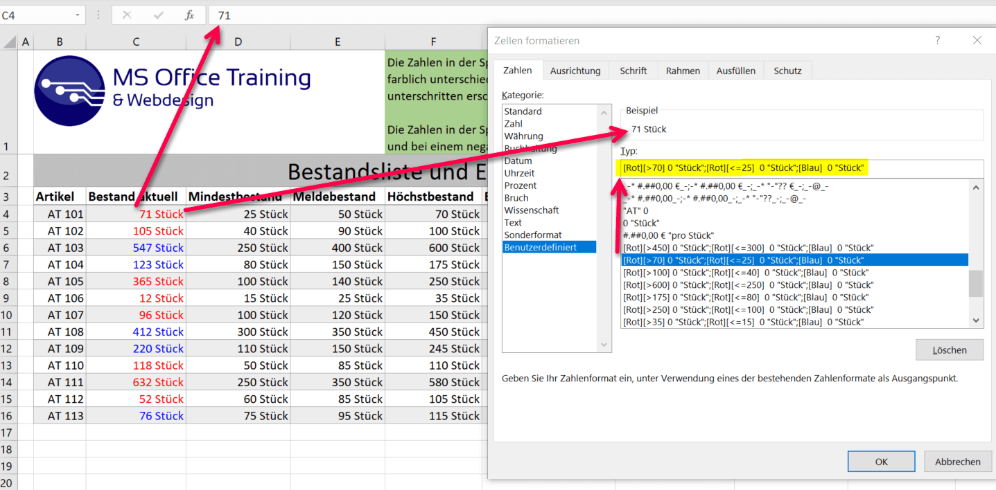
The numbers in the “Current stock” column should be formatted in such a way that they automatically appear in red if the stock exceeds the maximum stock or falls below the minimum stock, and otherwise in blue font. In addition, there should not only be the pure number, but the additional information “piece” after the number. So that this works, let’s take a look at the first row of the table:
The stock is currently 71 pieces, the minimum stock is 25 pieces and the maximum stock is 70 pieces. The maximum stock has thus been exceeded and the number is displayed in red. To do this, we used the following custom formatting:
see fig. (click to enlarge)
[Red][>70] 0 “pieces”;[Red][<=25] 0 “pieces”;[Blue] 0 “pieces”
Let’s break down our formatting into its individual parts for a better understanding:
1. [Red][>70] 0 “Piece” = The color value of the number is specified in the square brackets at the beginning, and in the second square bracket behind it we specify a condition for when this should be the case. Here the number should appear in red if the number is greater than 70. Next, we didn’t just want to have the pure number there, but the information “piece”. You can put text both before and after a number. So that Excel can calculate with it, you must ALWAYS put the text in “”!
2.;[Red][<=25] 0 “piece” = The first character we see is a semicolon. This is how we separate the sections within our conditional formatting code. You can use up to four sections within a format code, but you must always ensure that they are separated from one another with a semicolon so that the formatting works. So first we specify the color again, and then we specify the argument that this should be on condition that the number is less than or equal to 25.
3.;[Blue] 0 “Piece” = In the last section of our formatting, we specify that if none of the arguments mentioned above applies, the font should be blue, and of course our additional text “Piece”. If we left out the third section completely, Excel would only output the pure number in the default font color.
Note: In the screenshot above, you will have noticed that when you select cell C4, which says “71 pieces”, this information is not reflected in the formula bar. There is only the number 71. This is because by adding text in “” Excel can ignore this text and only look at the number. If we were to simply write 71 pieces into the cell without displaying this using formatting, Excel would treat the content of the cell as text. And you can’t calculate with text!
We hope that our little tutorial has given you a little more insight into custom formatting in Excel. And again, don’t be fooled by all the special characters that are already in the formatting options. You can use them, but you don’t have to. Now that you know what the characters mean, you can easily create your own custom formatting in Excel.
Tip: You can also find out more about cell formatting options in our tutorial on conditional formatting in Excel.
You can download the table that we used for this tutorial for free and try it out a bit.
Application examples of custom formatting
As already shown in the table, the numbers can be displayed as currency, fraction, and / or different decimal places and colors using the user-defined formatting in Excel. Times and dates can also be adjusted to the extent that Excel can calculate them. We have created an example table with different formatting, which we would like to use to explain some of the possibilities.
Note: This sample table can also be downloaded here for free >>>
In our table, we focus on a list of various current item stocks, as well as the reorder, minimum, and maximum stock levels of each item. In addition, the current acquisition prices, the maximum justifiable purchase prices, as well as sales prices per unit and the resulting positive and negative (loss) profit margins per unit.
The numbers in the “Current stock” column should be formatted in such a way that they automatically appear in red if the stock exceeds the maximum stock or falls below the minimum stock, and otherwise in blue font. In addition, there should not only be the pure number, but the additional information “piece” after the number. So that this works, let’s take a look at the first row of the table:
The stock is currently 71 pieces, the minimum stock is 25 pieces and the maximum stock is 70 pieces. The maximum stock has thus been exceeded and the number is displayed in red. To do this, we used the following custom formatting:
see fig. (click to enlarge)
[Red][>70] 0 “pieces”;[Red][<=25] 0 “pieces”;[Blue] 0 “pieces”
Let’s break down our formatting into its individual parts for a better understanding:
1. [Red][>70] 0 “Piece” = The color value of the number is specified in the square brackets at the beginning, and in the second square bracket behind it we specify a condition for when this should be the case. Here the number should appear in red if the number is greater than 70. Next, we didn’t just want to have the pure number there, but the information “piece”. You can put text both before and after a number. So that Excel can calculate with it, you must ALWAYS put the text in “”!
2.;[Red][<=25] 0 “piece” = The first character we see is a semicolon. This is how we separate the sections within our conditional formatting code. You can use up to four sections within a format code, but you must always ensure that they are separated from one another with a semicolon so that the formatting works. So first we specify the color again, and then we specify the argument that this should be on condition that the number is less than or equal to 25.
3.;[Blue] 0 “Piece” = In the last section of our formatting, we specify that if none of the arguments mentioned above applies, the font should be blue, and of course our additional text “Piece”. If we left out the third section completely, Excel would only output the pure number in the default font color.
Note: In the screenshot above, you will have noticed that when you select cell C4, which says “71 pieces”, this information is not reflected in the formula bar. There is only the number 71. This is because by adding text in “” Excel can ignore this text and only look at the number. If we were to simply write 71 pieces into the cell without displaying this using formatting, Excel would treat the content of the cell as text. And you can’t calculate with text!
We hope that our little tutorial has given you a little more insight into custom formatting in Excel. And again, don’t be fooled by all the special characters that are already in the formatting options. You can use them, but you don’t have to. Now that you know what the characters mean, you can easily create your own custom formatting in Excel.
Tip: You can also find out more about cell formatting options in our tutorial on conditional formatting in Excel.
You can download the table that we used for this tutorial for free and try it out a bit.
Popular Posts:

So sieht das wirklich perfekte Homeoffice-Setup für 2026 aus
Ihr Homeoffice ist veraltet? Steigern Sie 2026 Produktivität & Gesundheit. Unser Guide zeigt das perfekte Setup: von ergonomischen Stühlen und 4K-Webcams bis zu Mesh-WLAN und Kabelmanagement. So investieren Sie in Ihre Karriere.

Internet, Telefon & TV: Die besten Komplettpakete
Internet, TV & Telefon aus einer Hand? Wir vergleichen die Komplettpakete von Telekom, Vodafone, O2 & 1&1. Wer punktet bei Speed, TV-Komfort (MagentaTV vs. GigaTV) und Preis? So finden Sie das beste Triple-Play-Angebot für Ihre Adresse.

5 Anzeichen, dass dein Chef dich im Homeoffice digital überwacht
Nur weil du im Homeoffice bist, heißt das nicht, dass dir niemand zusieht. "Bossware" ist auf dem Vormarsch. Wir zeigen 5 subtile Anzeichen für digitale Überwachung – von "Teams-Status"-Kult bis zu verdächtigen IT-Tools. So erkennst du die Warnsignale und schützt deine Karriere.

Schluss mit dem Tool-Chaos: 5 Apps, die Euer Office wirklich produktiver machen
Schluss mit digitaler Reibung: Diese 5 Apps machen Ihr Büro wirklich produktiver. Entdecken Sie, wie Asana, Loom, Notion, Zapier und Slack die Effizienz steigern, Meetings reduzieren und Ihr Team smarter vernetzen – wenn man sie richtig einsetzt.

AI in everyday office life: Your new invisible colleague
AI won't replace you – but those who use it will have a competitive edge. Make AI your co-pilot in the office! We'll show you four concrete hacks for faster emails, better meeting notes, and solved Excel problems. Get started today, no IT degree required.

Fünf vor Zwölf: Wie Sie erkennen, dass Sie kurz vor dem Burnout stehen
Erschöpfung ist normal, doch wenn das Wochenende keine Erholung mehr bringt und Zynismus die Motivation ersetzt, stehen Sie kurz vor dem Burnout. Erfahren Sie, welche 7 Warnsignale Sie niemals ignorieren dürfen und warum es jetzt lebenswichtig ist, die Notbremse zu ziehen
Offers 2024: Word & Excel Templates


Popular Posts:
So sieht das wirklich perfekte Homeoffice-Setup für 2026 aus
Ihr Homeoffice ist veraltet? Steigern Sie 2026 Produktivität & Gesundheit. Unser Guide zeigt das perfekte Setup: von ergonomischen Stühlen und 4K-Webcams bis zu Mesh-WLAN und Kabelmanagement. So investieren Sie in Ihre Karriere.
Internet, Telefon & TV: Die besten Komplettpakete
Internet, TV & Telefon aus einer Hand? Wir vergleichen die Komplettpakete von Telekom, Vodafone, O2 & 1&1. Wer punktet bei Speed, TV-Komfort (MagentaTV vs. GigaTV) und Preis? So finden Sie das beste Triple-Play-Angebot für Ihre Adresse.
5 Anzeichen, dass dein Chef dich im Homeoffice digital überwacht
Nur weil du im Homeoffice bist, heißt das nicht, dass dir niemand zusieht. "Bossware" ist auf dem Vormarsch. Wir zeigen 5 subtile Anzeichen für digitale Überwachung – von "Teams-Status"-Kult bis zu verdächtigen IT-Tools. So erkennst du die Warnsignale und schützt deine Karriere.
Schluss mit dem Tool-Chaos: 5 Apps, die Euer Office wirklich produktiver machen
Schluss mit digitaler Reibung: Diese 5 Apps machen Ihr Büro wirklich produktiver. Entdecken Sie, wie Asana, Loom, Notion, Zapier und Slack die Effizienz steigern, Meetings reduzieren und Ihr Team smarter vernetzen – wenn man sie richtig einsetzt.
AI in everyday office life: Your new invisible colleague
AI won't replace you – but those who use it will have a competitive edge. Make AI your co-pilot in the office! We'll show you four concrete hacks for faster emails, better meeting notes, and solved Excel problems. Get started today, no IT degree required.
Fünf vor Zwölf: Wie Sie erkennen, dass Sie kurz vor dem Burnout stehen
Erschöpfung ist normal, doch wenn das Wochenende keine Erholung mehr bringt und Zynismus die Motivation ersetzt, stehen Sie kurz vor dem Burnout. Erfahren Sie, welche 7 Warnsignale Sie niemals ignorieren dürfen und warum es jetzt lebenswichtig ist, die Notbremse zu ziehen
Offers 2024: Word & Excel Templates