Apply nested functions in Excel
Most users are familiar with the simple functions in Excel. However, only a few know that functions in Excel can also be nested with one another. By nesting functions, Excel offers exactly the possibilities that cannot be mapped by the individual functions.
Nested functions in Excel can be mapped on up to 64 levels, and thus also enable very complex function models and application scenarios to be displayed. In our tutorial, we would like to take a quick look at how nested functions work in Excel.
Nesting and combining functions in Excel
In order to show the nesting and combining of functions in Excel as transparently as possible, we have created an example table. Customers should receive a predefined discount under various conditions. To do this, we nested an IF function and an OR function, and then again with an IF function and an AND function.
This allows different discounts to be displayed depending on the turnover made and an additional combination with the order quantity.
In the first example, we’ll look at combining an IF function with an AND function. The following conditions must be met for the customer to receive a discount:
The customer should receive a discount of 5% on the retail price if the order quantity is greater than 5 pieces. And this regardless of the turnover.
The customer should receive a discount of 10% on the retail price if the order quantity is greater than 5 pieces and the turnover is over €1,000.
If none of the conditions are met, the cell should say No discount.
see fig. (click to enlarge)
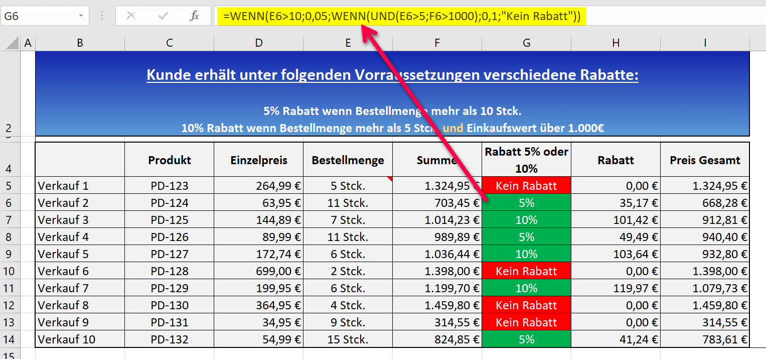

The full nested function in Excel looks like this to represent the desired discount or “No discount” notice:
=IF(E6>10;0,05;IF(AND(E6>5;F6>1000);0,1;”No discount”))
We will now take the function apart piece by piece for the sake of explanation
- =IF( = Here we open the IF function
- =IF(E6>10;0,05; = The first part of the function says that IF the order quantity is greater than 10 pieces THEN the order quantity is greater than 10 pieces THEN the cell there should be filled with the value 0.05. Due to the formatting of the cell as a percentage value there later 5% displayed correctly.
- IF(AND( = Instead of supplying the value for ELSE as usual with an IF function, we immediately insert the next IF function and combine it with an AND function.
- E6>5;F6>1000) = With the AND-function we specify additional arguments that must be fulfilled in order to receive the 10% discount. In this part of the function we say that IF the order quantity is greater than 5 pieces, AND the purchase Value is over 1.000€ than… From here we close the AND function again with the brackets.
- ;0,1;”No discount”)) = In the last part of the function, we continue the IF function we started at the beginning, and state the steps that Excel should take if the two arguments that must be fulfilled for the 10% are true . So if the quantity is more than 5 pieces and the sales price is more than €1,000, the cell should be filled with the value 0.1, and if the two arguments do not apply together, “No discount” should appear there. With the two parentheses at the end, we close our nested function.
Here again the fully nested IF AND function with which both 5%, 10% and also the note “No discount” can be displayed.
=IF(E6>10;0,05;IF(AND(E6>5;F6>1000);0,1;”No discount”))
By the way:
You can automate the colored markings in the column with the percentage values and the note “No discount” with conditional formatting in Excel. Click here for the article
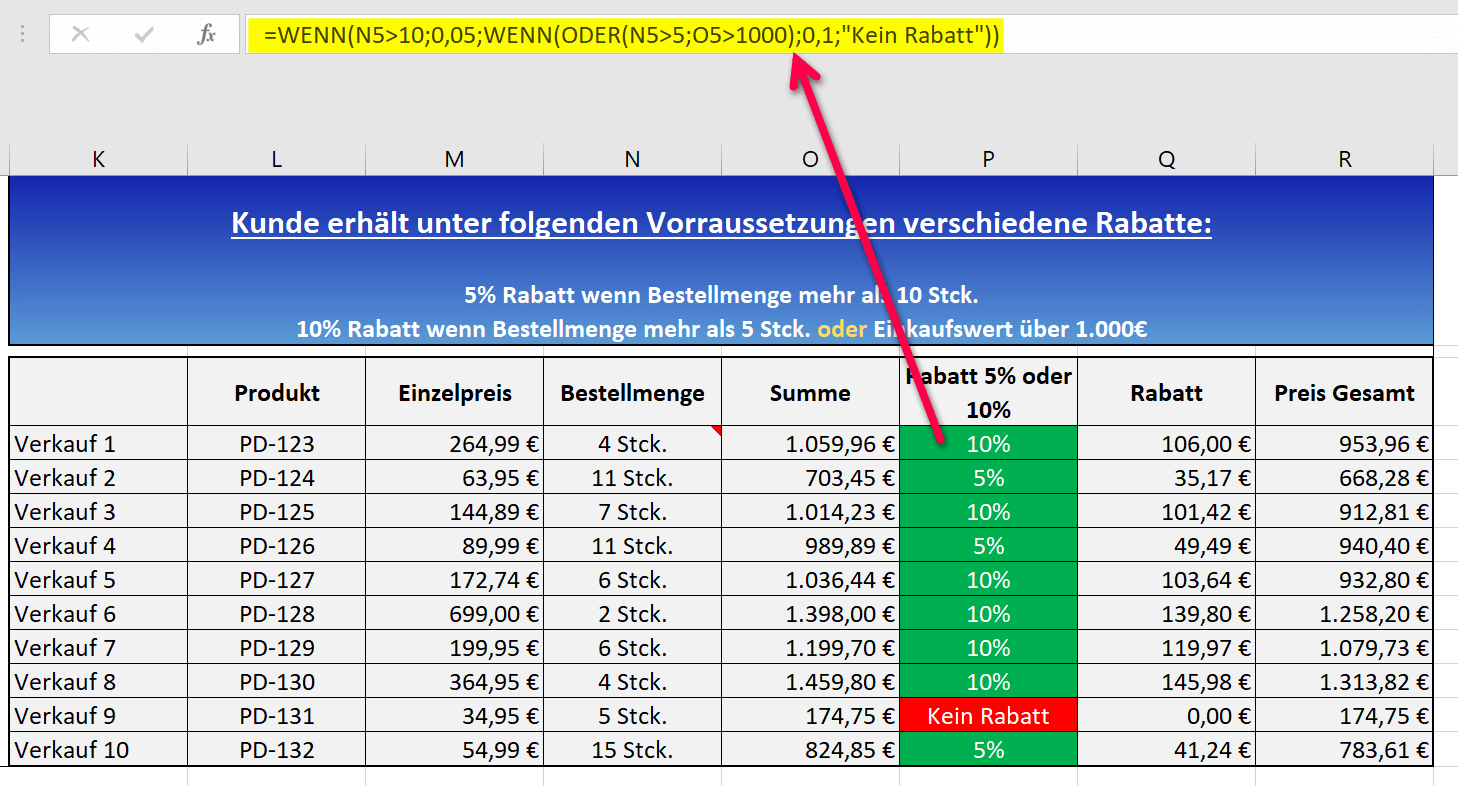
Of course, you can also combine the whole thing with an IF-OR function, in which, for example, not several conditions, but only one of the two (or more) must be fulfilled in order to receive a corresponding discount, or even the message “No discount”.
The nested function in Excel would then look like this:
=IF(N5>10;0,05;IF(OR(N5>5;O5>1000);0,1;”No discount”))
siehe Abb. (klicken zum vergrößern)
You can download the Excel file that we have built to illustrate the facts clearly here for free to experiment with it.
Nesting and combining functions in Excel
In order to show the nesting and combining of functions in Excel as transparently as possible, we have created an example table. Customers should receive a predefined discount under various conditions. To do this, we nested an IF function and an OR function, and then again with an IF function and an AND function.
This allows different discounts to be displayed depending on the turnover made and an additional combination with the order quantity.
In the first example, we’ll look at combining an IF function with an AND function. The following conditions must be met for the customer to receive a discount:
The customer should receive a discount of 5% on the retail price if the order quantity is greater than 5 pieces. And this regardless of the turnover.
The customer should receive a discount of 10% on the retail price if the order quantity is greater than 5 pieces and the turnover is over €1,000.
If none of the conditions are met, the cell should say No discount.
see fig. (click to enlarge)
The full nested function in Excel looks like this to represent the desired discount or “No discount” notice:
=IF(E6>10;0,05;IF(AND(E6>5;F6>1000);0,1;”No discount”))
We will now take the function apart piece by piece for the sake of explanation
- =IF( = Here we open the IF function
- =IF(E6>10;0,05; = The first part of the function says that IF the order quantity is greater than 10 pieces THEN the order quantity is greater than 10 pieces THEN the cell there should be filled with the value 0.05. Due to the formatting of the cell as a percentage value there later 5% displayed correctly.
- IF(AND( = Instead of supplying the value for ELSE as usual with an IF function, we immediately insert the next IF function and combine it with an AND function.
- E6>5;F6>1000) = With the AND-function we specify additional arguments that must be fulfilled in order to receive the 10% discount. In this part of the function we say that IF the order quantity is greater than 5 pieces, AND the purchase Value is over 1.000€ than… From here we close the AND function again with the brackets.
- ;0,1;”No discount”)) = In the last part of the function, we continue the IF function we started at the beginning, and state the steps that Excel should take if the two arguments that must be fulfilled for the 10% are true . So if the quantity is more than 5 pieces and the sales price is more than €1,000, the cell should be filled with the value 0.1, and if the two arguments do not apply together, “No discount” should appear there. With the two parentheses at the end, we close our nested function.
Here again the fully nested IF AND function with which both 5%, 10% and also the note “No discount” can be displayed.
=IF(E6>10;0,05;IF(AND(E6>5;F6>1000);0,1;”No discount”))
By the way:
You can automate the colored markings in the column with the percentage values and the note “No discount” with conditional formatting in Excel. Click here for the article
Of course, you can also combine the whole thing with an IF-OR function, in which, for example, not several conditions, but only one of the two (or more) must be fulfilled in order to receive a corresponding discount, or even the message “No discount”.
The nested function in Excel would then look like this:
=IF(N5>10;0,05;IF(OR(N5>5;O5>1000);0,1;”No discount”))
siehe Abb. (klicken zum vergrößern)
You can download the Excel file that we have built to illustrate the facts clearly here for free to experiment with it.
Popular Posts:

Dynamic ranges in Excel: OFFSET function
The OFFSET function in Excel creates a flexible reference. Instead of fixing =SUM(B5:B7), the function finds the range itself, e.g., for the "last 3 months". Ideal for dynamic charts or dashboards that grow automatically.

Mastering the INDIRECT function in Excel
The INDIRECT function in Excel converts text into a real reference. Instead of manually typing =January!E10, use =INDIRECT(A2 & "!E10"), where A2 contains 'January'. This allows you to easily create dynamic summaries for multiple worksheets.

From assistant to agent: Microsoft’s Copilot
Copilot is growing up: Microsoft's AI is no longer an assistant, but a proactive agent. With "Vision," it sees your Windows desktop; in M365, it analyzes data as a "Researcher"; and in GitHub, it autonomously corrects code. The biggest update yet.

Windows 12: Where is it? The current status in October 2025
Everyone was waiting for Windows 12 in October 2025, but it didn't arrive. Instead, Microsoft is focusing on Windows 11 25H2 and "Copilot+ PC" features. We'll explain: Is Windows 12 canceled, postponed, or is it already available as an AI update for Windows 11?

Blocking websites on Windows using the hosts file
Want to block unwanted websites in Windows? You can do it without extra software using the hosts file. We'll show you how to edit the file as an administrator and redirect domains like example.de to 127.0.0.1. This will block them immediately in all browsers.

The “Zero Inbox” method with Outlook: How to permanently get your mailbox under control.
Caught red-handed? Your Outlook inbox has 1000+ emails? That's pure stress. Stop the email deluge with the "Zero Inbox" method. We'll show you how to clean up your inbox and regain control using Quick Steps and rules.
Offers 2024: Word & Excel Templates


Popular Posts:
Dynamic ranges in Excel: OFFSET function
The OFFSET function in Excel creates a flexible reference. Instead of fixing =SUM(B5:B7), the function finds the range itself, e.g., for the "last 3 months". Ideal for dynamic charts or dashboards that grow automatically.
Mastering the INDIRECT function in Excel
The INDIRECT function in Excel converts text into a real reference. Instead of manually typing =January!E10, use =INDIRECT(A2 & "!E10"), where A2 contains 'January'. This allows you to easily create dynamic summaries for multiple worksheets.
From assistant to agent: Microsoft’s Copilot
Copilot is growing up: Microsoft's AI is no longer an assistant, but a proactive agent. With "Vision," it sees your Windows desktop; in M365, it analyzes data as a "Researcher"; and in GitHub, it autonomously corrects code. The biggest update yet.
Windows 12: Where is it? The current status in October 2025
Everyone was waiting for Windows 12 in October 2025, but it didn't arrive. Instead, Microsoft is focusing on Windows 11 25H2 and "Copilot+ PC" features. We'll explain: Is Windows 12 canceled, postponed, or is it already available as an AI update for Windows 11?
Blocking websites on Windows using the hosts file
Want to block unwanted websites in Windows? You can do it without extra software using the hosts file. We'll show you how to edit the file as an administrator and redirect domains like example.de to 127.0.0.1. This will block them immediately in all browsers.
The “Zero Inbox” method with Outlook: How to permanently get your mailbox under control.
Caught red-handed? Your Outlook inbox has 1000+ emails? That's pure stress. Stop the email deluge with the "Zero Inbox" method. We'll show you how to clean up your inbox and regain control using Quick Steps and rules.
Offers 2024: Word & Excel Templates