Clean up Excel spreadsheets
If you have created an Excel table and it becomes more and more confusing over time, and perhaps some errors such as double entries have crept in, the whole thing must first be cleaned up in order to get a clear view again. Sometimes, however, you are presented with catastrophic tables created without a system, with the task of extracting usable data from them.
It helps if you know one or the other trick to make the whole thing go a little faster.

And that’s exactly what this little tutorial is supposed to be about today. We share 4 extremely helpful ways to do things like remove duplicates in Excel, delete blank cells, and fix texts in a few simple steps. This can save you the day with very large Excel spreadsheets and free up space for other things.
Clean up Excel spreadsheets
If you have created an Excel table and it becomes more and more confusing over time, and perhaps some errors such as double entries have crept in, the whole thing must first be cleaned up in order to get a clear view again. Sometimes, however, you are presented with catastrophic tables created without a system, with the task of extracting usable data from them.
It helps if you know one or the other trick to make the whole thing go a little faster.
And that’s exactly what this little tutorial is supposed to be about today. We share 4 extremely helpful ways to do things like remove duplicates in Excel, delete blank cells, and fix texts in a few simple steps. This can save you the day with very large Excel spreadsheets and free up space for other things.
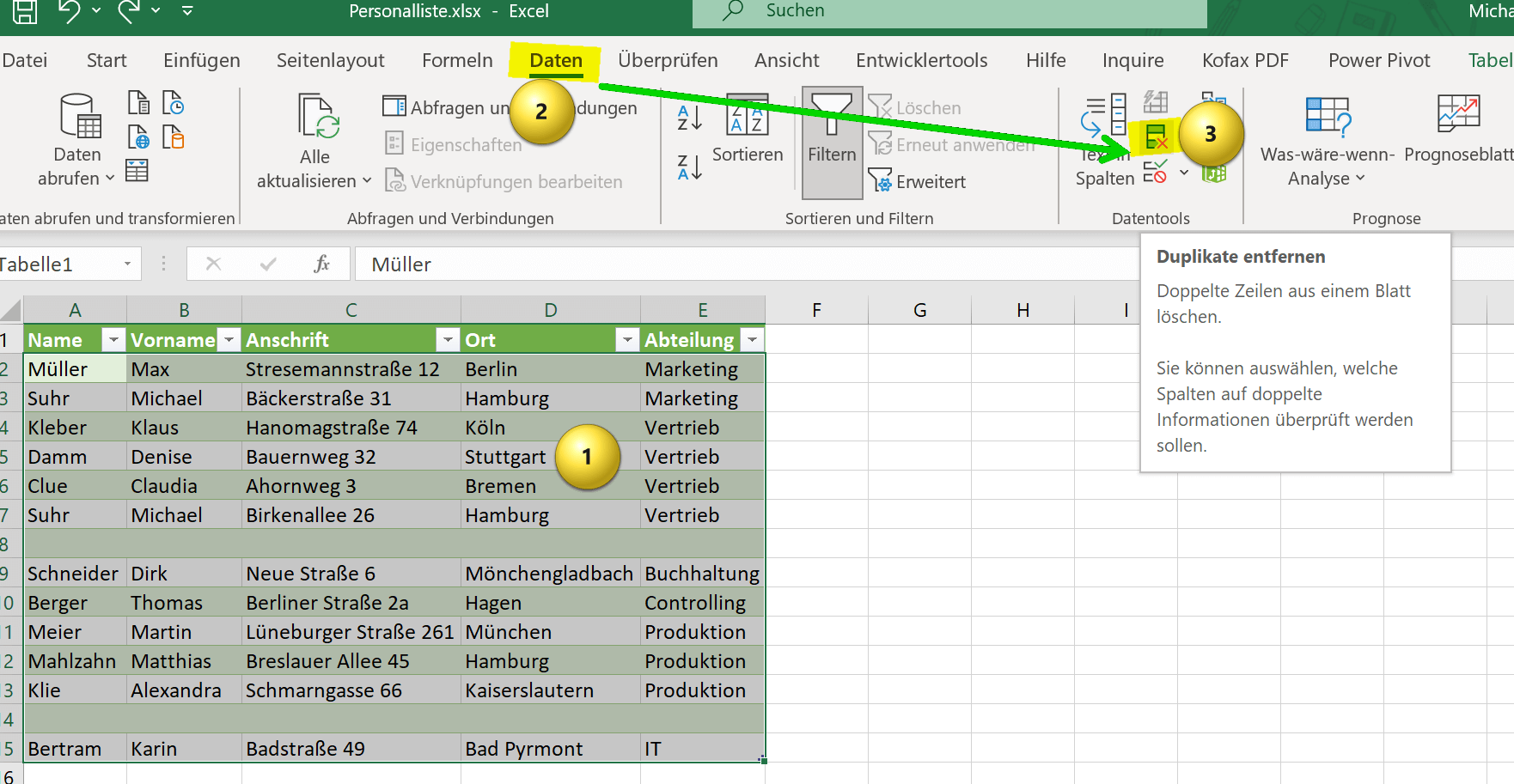
Remove duplicates in Excel
Remove duplicates in Excel
There are different ways to remove duplicates in Excel, depending on which version of Excel you are using. Here are three options:
Option 1: Remove duplicates using Excel’s Remove Duplicates feature
- Select the area where you want to remove duplicates.
- Click on the “Data” tab in the menu bar.
- Click “Remove Duplicates“.
- Check the box next to the columns that may contain duplicates.
- Click “OK“.
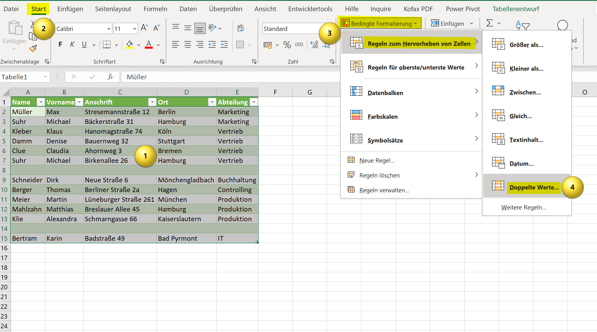
Option 2: Remove Duplicates Using Excel’s Conditional Formatting Feature
- Select the area where you want to remove duplicates.
- Click on the “Start” tab in the menu bar.
- Click Conditional Formatting.
- Click Highlight Cell Rules, then click “Remove Duplicates“.
- Check the box next to the columns that may contain duplicates.
- Click “OK“.
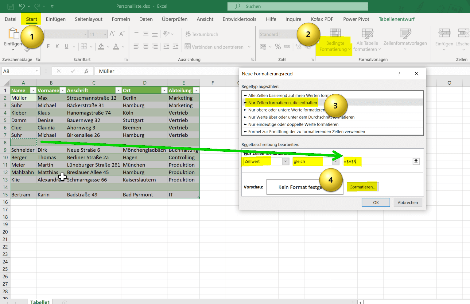
Option 3: Remove duplicates with a formula
To remove duplicates in Excel using a formula, you can combine the “COUNTIF” and “IF” function.
- First, mark the column or areas where you want to remove duplicates.
- Then create a new column next to the highlighted column.
- In the first cell of the new column, enter the following formula: =IF(COUNTIF(A:A,A1)>1,”Duplicate”,”Unique”)
(If your data is in a column other than column A, you must change the column label in the formula accordingly.) - Drag the formula down to apply it to all cells in the new column.
Now filter the new column for “duplicate” and delete the corresponding rows.
The formula above compares each cell in the selected column to all other cells in the same column and counts the number of occurrences of each cell. If a cell occurs more than once, the new column will say “Duplicate“, otherwise “Unique“. You can then filter by “duplicate” to select and delete all rows with duplicates.
see fig.(click to enlarge)

There are different ways to remove duplicates in Excel, depending on which version of Excel you are using. Here are three options:
Option 1: Remove duplicates using Excel’s Remove Duplicates feature
- Select the area where you want to remove duplicates.
- Click on the “Data” tab in the menu bar.
- Click “Remove Duplicates“.
- Check the box next to the columns that may contain duplicates.
- Click “OK“.
Option 2: Remove Duplicates Using Excel’s Conditional Formatting Feature
- Select the area where you want to remove duplicates.
- Click on the “Start” tab in the menu bar.
- Click Conditional Formatting.
- Click Highlight Cell Rules, then click “Remove Duplicates“.
- Check the box next to the columns that may contain duplicates.
- Click “OK“.
Option 3: Remove duplicates with a formula
To remove duplicates in Excel using a formula, you can combine the “COUNTIF” and “IF” function.
- First, mark the column or areas where you want to remove duplicates.
- Then create a new column next to the highlighted column.
- In the first cell of the new column, enter the following formula: =IF(COUNTIF(A:A,A1)>1,”Duplicate”,”Unique”)
(If your data is in a column other than column A, you must change the column label in the formula accordingly.) - Drag the formula down to apply it to all cells in the new column.
Now filter the new column for “duplicate” and delete the corresponding rows.
The formula above compares each cell in the selected column to all other cells in the same column and counts the number of occurrences of each cell. If a cell occurs more than once, the new column will say “Duplicate“, otherwise “Unique“. You can then filter by “duplicate” to select and delete all rows with duplicates.
see fig.(click to enlarge)
Remove empty cells in Excel
Remove empty cells in Excel
To remove blank cells in Excel, there are different ways depending on which version of Excel you are using. Here are two options:
Option 1: Remove blank cells using Excel’s Conditional Formatting feature
- Select the range where you want to remove blank cells.
- Click on the “Start” tab in the menu bar.
- Click Conditional Formatting.
- Click “New Rule” and then “Format only cells that contain“.
- From the Cell Value drop-down menu, choose equals and click in the box to the right of it.
- Then click in any cell within your spreadsheet that is empty.
- Choose a format for the blank cells to be selected, e.g. B. a background color.
- Click “OK“.
- Select and delete the marked blank cells.
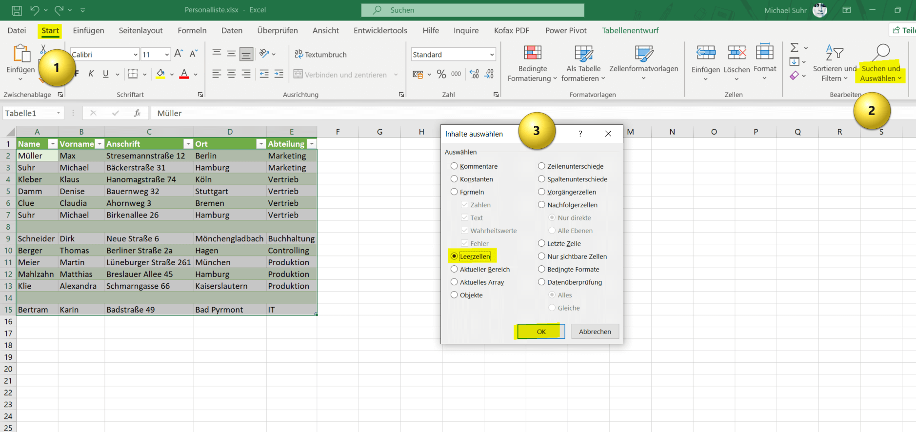
Option 2: Remove Blank Cells Using Find Function
To remove blank cells using find function in Excel, you can follow the steps below:
- Mark the relevant table in which the check is to take place.
- From the “Home” tab, go to “Find and Select” and then to “Go“
- In the dialog window, select “Content” at the bottom left.
- Here you now have various options to search for and select content within your selected table.
- So select “Empty Cells” here and confirm with “OK“
- Now all empty cells in your spreadsheet will be highlighted and you can simply delete them by pressing “DEL” on your keyboard.
see fig.(click to enlarge)
To remove blank cells in Excel, there are different ways depending on which version of Excel you are using. Here are two options:
Option 1: Remove blank cells using Excel’s Conditional Formatting feature
- Select the range where you want to remove blank cells.
- Click on the “Start” tab in the menu bar.
- Click Conditional Formatting.
- Click “New Rule” and then “Format only cells that contain“.
- From the Cell Value drop-down menu, choose equals and click in the box to the right of it.
- Then click in any cell within your spreadsheet that is empty.
- Choose a format for the blank cells to be selected, e.g. B. a background color.
- Click “OK“.
- Select and delete the marked blank cells.
Option 2: Remove Blank Cells Using Find Function
To remove blank cells using find function in Excel, you can follow the steps below:
- Mark the relevant table in which the check is to take place.
- From the “Home” tab, go to “Find and Select” and then to “Go“
- In the dialog window, select “Content” at the bottom left.
- Here you now have various options to search for and select content within your selected table.
- So select “Empty Cells” here and confirm with “OK“
- Now all empty cells in your spreadsheet will be highlighted and you can simply delete them by pressing “DEL” on your keyboard.
see fig.(click to enlarge)
Remove formatting in Excel
Remove formatting in Excel
To quickly remove formatting in Excel, do the following:
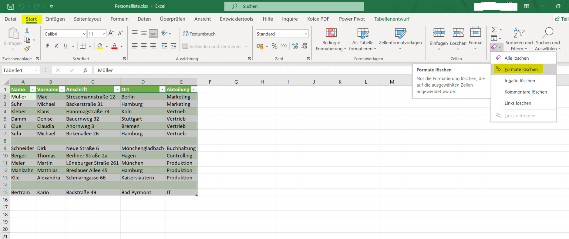
- Select the area to remove formatting.
- Then go to the “Edit” section on the far right via the “Home” tab and select the sub-item “Clear Formats“.
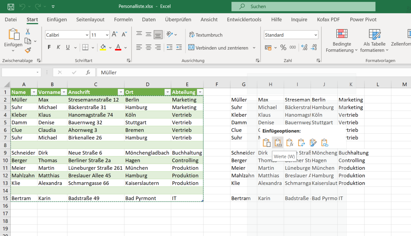
- The second option would be to mark the desired table area and then copy it with the key combination “CTRL+C“.
- Then click in a free area of your spreadsheet or use a new one, and then select “Values” from the context menu under “Insert“.
- In this way, the pure cell values are copied without any formatting.
see fig.(click to enlarge)
To quickly remove formatting in Excel, do the following:
- Select the area to remove formatting.
- Then go to the “Edit” section on the far right via the “Home” tab and select the sub-item “Clear Formats“.
- The second option would be to mark the desired table area and then copy it with the key combination “CTRL+C“.
- Then click in a free area of your spreadsheet or use a new one, and then select “Values” from the context menu under “Insert“.
- In this way, the pure cell values are copied without any formatting.
see fig.(click to enlarge)
Clean up texts in Excel
Clean up texts in Excel
To perform text cleanup in Excel, we would like to offer two ways:
Possibility Number 1:
- Highlight the area where you want to perform text cleanup.
- Click on the “Data” tab and then click on the “Text to Columns” button in the “Data Tools” section.
- In the Text Conversion Wizard, select the Delimited option and click Next.
- Select the delimiters used in your text, such as space, tab, or comma, and click Next.
- Select the appropriate data format for each column. For example, for a column of dates, you can choose the date format.
- Click “Finish” to convert the data.
Possibility 2:
- Use Excel’s Find and Replace feature to remove or replace specific strings or characters in text.
- Click the Find and Replace button in the Edit section of the Home tab.
- Enter the string of characters you want to find or the character that you want to replace, and then enter the new text.
- Click Replace to remove or replace all occurrences of the string or character.
- Save the file with the cleaned data.
By following these steps, you can clean up text in Excel and format your data cleanly and consistently.
Popular Posts:

Excel Scenario manager and target value search
How you can use the scenario manager and target value search in Excel 2016/2019 to present complex issues in a space-saving and clear way.

Insert controls and form fields in Word
With Microsoft Word you can not only comfortably create letters, lists and articles with tables of contents, but also go one step further, and Set up your own forms using controls.

Apply nested functions in Excel
Nested functions in Excel offer the possibility to combine several arguments with each other or to exclude conditions. We explain how it works.

Save Emails and contacts as pst file in Outlook
Your emails and contacts are valuable, and not so easy to get back! Create a backup of your Outlook files in 5 steps.

Office 2021 – Everything you need to know about price, versions and scope
Shortly before the release, Microsoft announced the prices and scope for the new Office 2021. We are a little amazed at what is coming.

Insert Excel spreadsheets into Word Documents
So you can easily insert Excel spreadsheets into Word and link them together to get a dynamic document.
Offers 2024: Word & Excel Templates


Popular Posts:
Excel Scenario manager and target value search
How you can use the scenario manager and target value search in Excel 2016/2019 to present complex issues in a space-saving and clear way.
Insert controls and form fields in Word
With Microsoft Word you can not only comfortably create letters, lists and articles with tables of contents, but also go one step further, and Set up your own forms using controls.
Apply nested functions in Excel
Nested functions in Excel offer the possibility to combine several arguments with each other or to exclude conditions. We explain how it works.
Save Emails and contacts as pst file in Outlook
Your emails and contacts are valuable, and not so easy to get back! Create a backup of your Outlook files in 5 steps.
Office 2021 – Everything you need to know about price, versions and scope
Shortly before the release, Microsoft announced the prices and scope for the new Office 2021. We are a little amazed at what is coming.
Insert Excel spreadsheets into Word Documents
So you can easily insert Excel spreadsheets into Word and link them together to get a dynamic document.
Offers 2024: Word & Excel Templates