How does Conditional Formatting work in Excel
Many times, you have certainly wished that certain contents of your Excel spreadsheet be highlighted a little bit more, so that they catch your eye at a glance.
This is basically (as long as you do it statically) no problem and relatively easy to implement. After all, you can color any cell as you like, and make it larger or smaller as well. However, what we really want is that cells automatically get a pre-determined look under certain conditions.
How to use Conditional Formatting in Microsoft Excel can be found in our article.
1. What is Conditional Formatting in Excel?
1. What is Conditional Formatting in Excel?
First of all, let’s clarify the general question of what “conditional formatting” actually is.
As the name already implies, this is a cell formatting that under certain conditions takes place automatically. So we can e.g. The table says that if a cell contains a predetermined value, or if it is within a certain range, that cell will be highlighted in color.
So suppose you make yourself a household table, and there you have a job that usually always moves between 80 € and 100 € per month. However, the longer you run this list, the harder it will be to catch up on deviations at a glance.
However, if you add a “Conditional Formatting” to these cells, for example, once the value exceeds $ 100, you could automatically have Excel highlight that cell with a red background color.
Of course, this is first of all a bit of work, but it’s a job you do just once, and then the process runs automatically.
2. Predefined rules for conditional formatting
2. Predefined rules for conditional formatting
Now we come to the point.
In our first example, let’s look at the simplest discipline of conditional formatting in the form of predefined rules, and we have built up a sample table of budget expenditures for a year in which some values deviate from the usual ones that we get in the case of an increased amount red, and color at a lower amount with a green background.
To do this, we proceed as follows:
- The first line of the table in which the numerical values that should be considered for formatting should be highlighted.
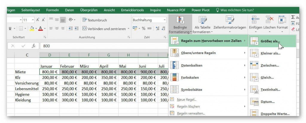
- In the “Start” tab, click on “Conditional Formatting” and click on “Highlight Rules” – “Greater than”.
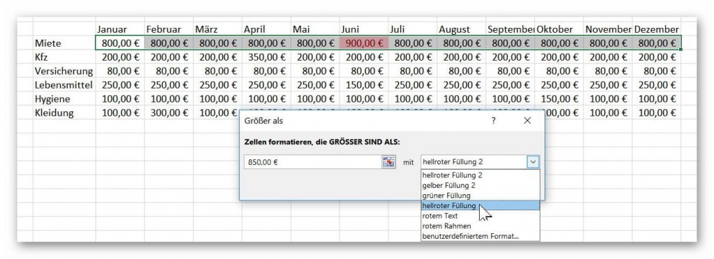
- Then set the upper threshold and the color from which the formatting to be held.
Then again the same game, only that we click here on “less than” a lower threshold and a corresponding color set.
See picture: (click to enlarge)
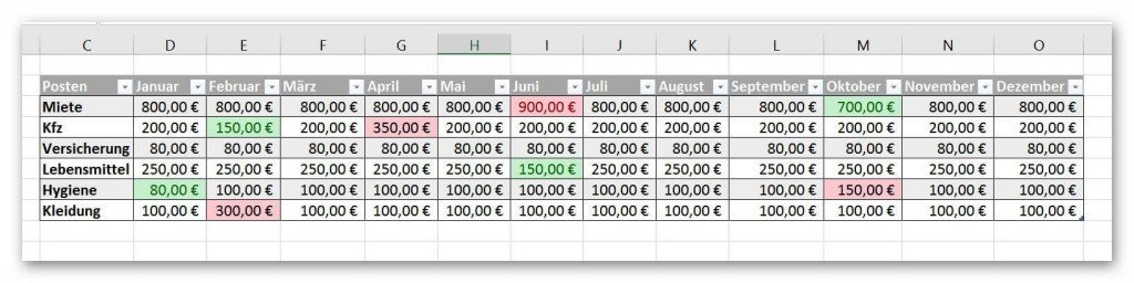
Thus, after we have set the thresholds for each item, our table looks like this in the end result:
See picture: (click to enlarge)

For example, if you create a household table at the beginning of the year and set thresholds for each item, Excel will automatically check whether the cell is colored or not when you enter it using Conditional Formatting.
This allows you to detect deviations at a glance without having to filter data or have to look through it manually.
Now we come to the point.
In our first example, let’s look at the simplest discipline of conditional formatting in the form of predefined rules, and we have built up a sample table of budget expenditures for a year in which some values deviate from the usual ones that we get in the case of an increased amount red, and color at a lower amount with a green background.
To do this, we proceed as follows:
- The first line of the table in which the numerical values that should be considered for formatting should be highlighted.
- In the “Start” tab, click on “Conditional Formatting” and click on “Highlight Rules” – “Greater than”.
- Then set the upper threshold and the color from which the formatting to be held.
Then again the same game, only that we click here on “less than” a lower threshold and a corresponding color set.
See picture:


Thus, after we have set the thresholds for each item, our table looks like this in the end result:
See picture:

For example, if you create a household table at the beginning of the year and set thresholds for each item, Excel will automatically check whether the cell is colored or not when you enter it using Conditional Formatting.
This allows you to detect deviations at a glance without having to filter data or have to look through it manually.
3. Conditional formatting with own rules
3. Conditional formatting with own rules
In our next example we want to go off the beaten path and set our own rules for conditional formatting.
For the sake of simplicity, we will stick with our small household table and will display all duplicate values in bold.
To do this, we proceed as follows:
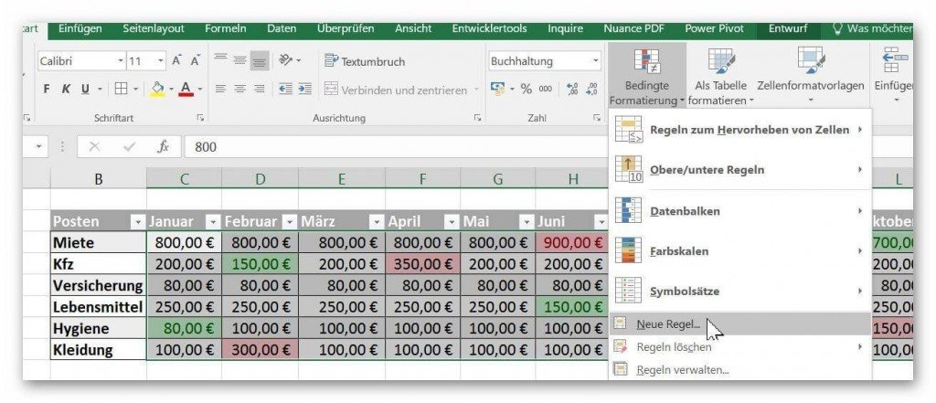
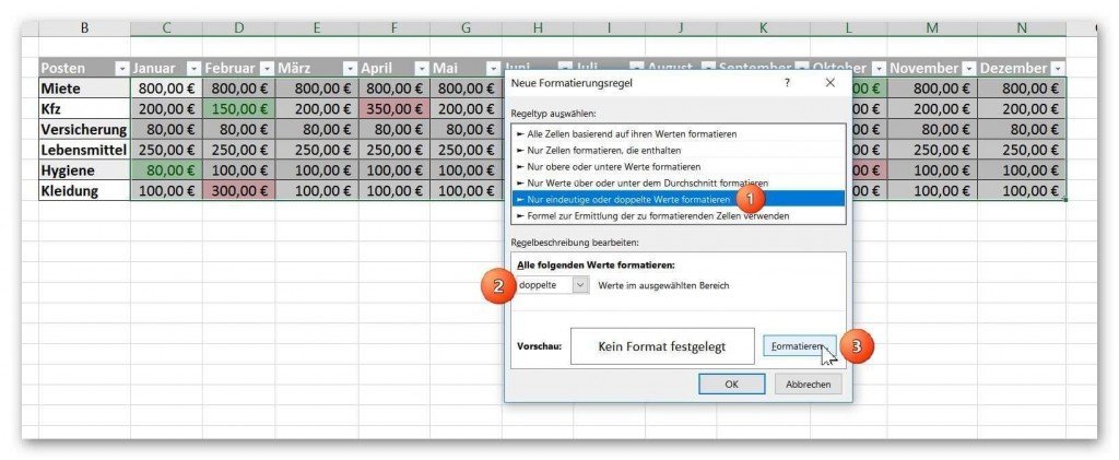
- We mark the entire cell area of the table which in the formatting should be considered.
- Then we click again on “Conditional Formatting” then on “New Rule” and select the option “Format only unique or duplicate values”
See picture: (click to enlarge)
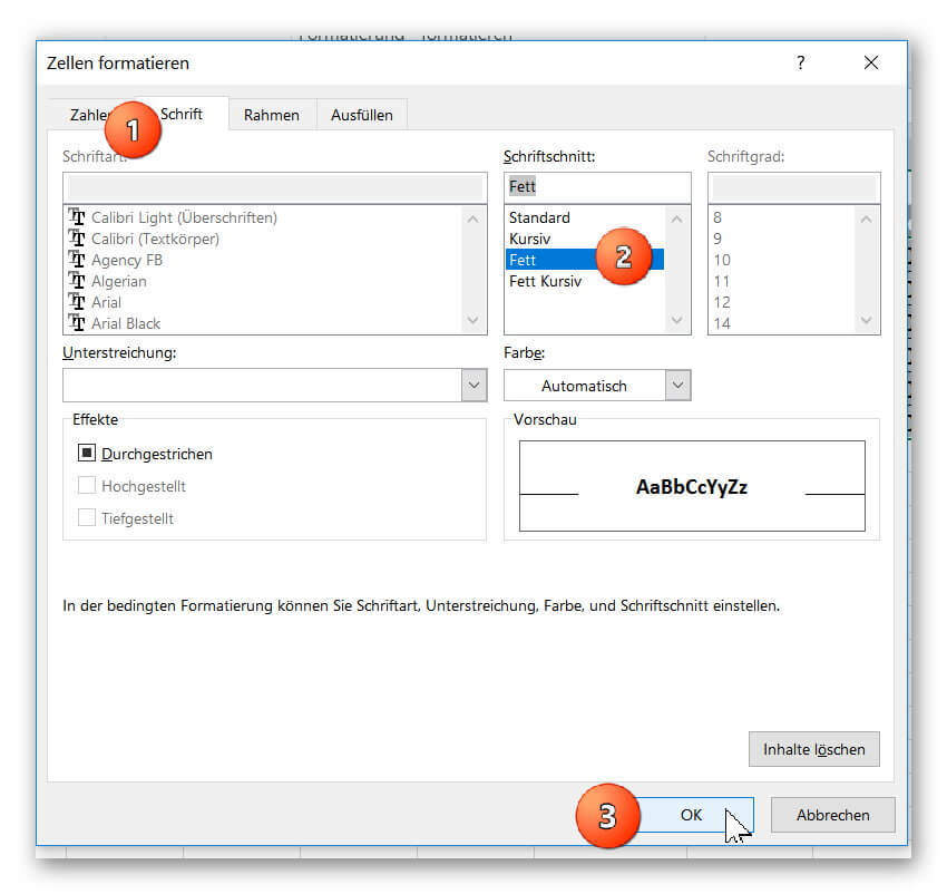
Then on “Format” and in the tab “Font” we choose FAT and confirm with “OK”.
See picture: (click to enlarge)
In our next example we want to go off the beaten path and set our own rules for conditional formatting.
For the sake of simplicity, we will stick with our small household table and will display all duplicate values in bold.
To do this, we proceed as follows:
- We mark the entire cell area of the table which in the formatting should be considered.
- Then we click again on “Conditional Formatting” then on “New Rule” and select the option “Format only unique or duplicate values”
See picture: (click to enlarge)
Then on “Format” and in the tab “Font” we choose FAT and confirm with “OK”.
See picture:
Popular Posts:

Import Stock Quotes into Excel – Tutorial
Importing stock quotes into Excel is not that difficult. And you can do a lot with it. We show you how to do it directly without Office 365.

Create Excel Budget Book – with Statistics – Tutorial
Create your own Excel budget book with a graphical dashboard, statistics, trends and data cut-off. A lot is possible with pivot tables and pivot charts.
Excel random number generator – With Analysis function
You can create random numbers in Excel using a function. But there are more possibilities with the analysis function in Excel.
Excel Database with Input Form and Search Function
So erstellen Sie eine Datenbank mit Eingabemaske und Suchfunktion OHNE VBA KENNTNISSE in Excel ganz einfach. Durch eine gut versteckte Funktion in Excel geht es recht einfach.

Enable developer tools in Office 365
Unlock developer tools in Excel, Word and Outlook. Expand the possibilities with additional functions in Office 365.
Dictate text in Word and have it typed
Dictating text in Word is much easier and faster than typing everything on the keyboard. Speech recognition in Word works just like external speech recognition software.
Offers 2024: Word & Excel Templates


Popular Posts:
Import Stock Quotes into Excel – Tutorial
Importing stock quotes into Excel is not that difficult. And you can do a lot with it. We show you how to do it directly without Office 365.
Create Excel Budget Book – with Statistics – Tutorial
Create your own Excel budget book with a graphical dashboard, statistics, trends and data cut-off. A lot is possible with pivot tables and pivot charts.
Excel random number generator – With Analysis function
You can create random numbers in Excel using a function. But there are more possibilities with the analysis function in Excel.
Excel Database with Input Form and Search Function
So erstellen Sie eine Datenbank mit Eingabemaske und Suchfunktion OHNE VBA KENNTNISSE in Excel ganz einfach. Durch eine gut versteckte Funktion in Excel geht es recht einfach.
Enable developer tools in Office 365
Unlock developer tools in Excel, Word and Outlook. Expand the possibilities with additional functions in Office 365.
Dictate text in Word and have it typed
Dictating text in Word is much easier and faster than typing everything on the keyboard. Speech recognition in Word works just like external speech recognition software.
Offers 2024: Word & Excel Templates