Excel Tutorial: How to quickly and safely remove duplicates

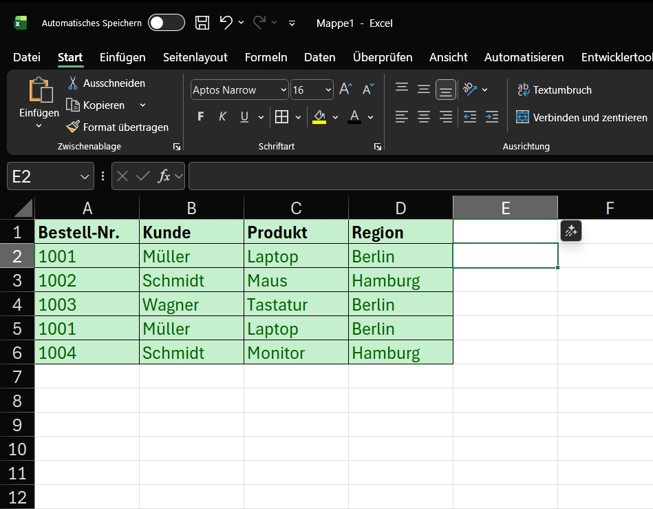
Imagine we have the following table with order data. We immediately see that some entries are repeated.

Our example data (range A1:D6):

Goals:

• Goal A: We want to remove exactly identical rows (row 5 is a duplicate of row 2).
• Goal B: We want to obtain a unique list of all customers (Müller, Schmidt, Wagner).

The “Remove Duplicates” function permanently deletes data.

⚠️ Important Security Note: Before you begin, always copy your worksheet or create a backup of your file. This way, if you make a mistake, you can revert to the original.

Step 1: Select the Data Range

• Click in your data table. Excel usually detects the contiguous range automatically. However, the safest method is to manually select the entire range (in our example, A1:D6) with your mouse.

Step 2: Finding the Function

• Go to the “Data” tab in the ribbon.
• Find the “Data Tools” group.
• Click the “Remove Duplicates” icon.

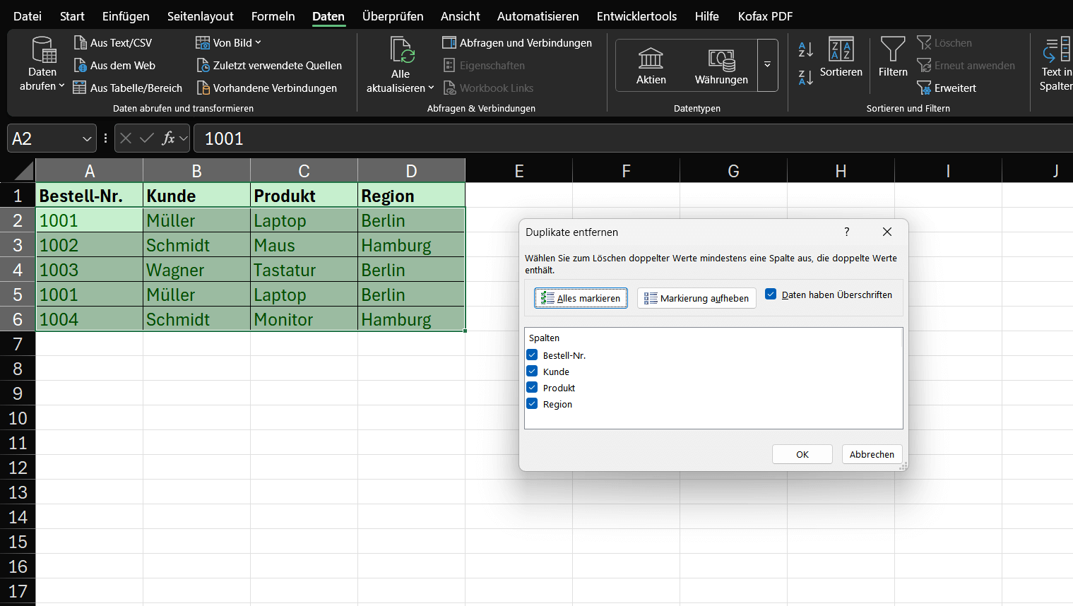
Step 3: The Dialog Box (The Most Important Step)

• A small window will open. This is the control center for the deletion process.
• “Data has headers”: Since our table has headers in row 1 (Order No., Customer, etc.), be sure to leave this checkbox selected. Excel will then ignore this row when deleting.
• Columns: Here, Excel lists all the columns from your selection.
  … This is where Excel decides what it considers a “duplicate”.

Scenario A: Deleting Exactly Identical Rows

Goal: We want to delete only row 5, as it is identical to row 2 in every column.

• Open “Remove Duplicates” (as described in steps 1 & 2).
• In the dialog box (step 3), ensure that ALL columns (Order No., Customer, Product, Region) are checked.
• Click “OK”.

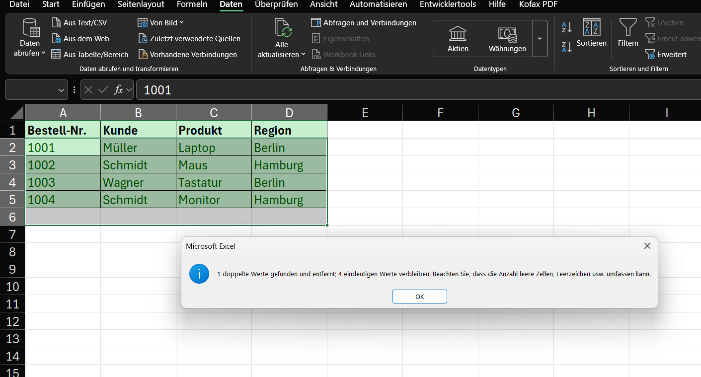
Result: Excel compares entire rows. Since only row 5 is an exact match for row 2, it is deleted. Excel reports: “1 duplicate found and removed; 4 unique values ​​remain.”

Note: Row 6 (Schmidt, Monitor) is NOT deleted, as it differs (in the product field) from row 3 (Schmidt, Mouse).

Scenario B: Creating a unique list based on ONE column

Goal: We are not interested in the entire table. We only want a unique list of all customers (Müller, Schmidt, Wagner).

• Open “Remove Duplicates”.
• In the dialog box, first click “Deselect” to remove all checkmarks.
• Check only the column you want to check for uniqueness – in our case, “Customer”.
• Click “OK”.

Result: Excel only looks in column B.

• Row 2 “Müller” is kept.
• Row 3 “Schmidt” is kept.
• Row 4 “Wagner” is kept.
• Row 5 “Müller” (duplicate!) is deleted.
• Row 6 “Schmidt” (duplicate!) is deleted.
• Excel reports: “2 duplicates Found and removed; 3 unique values ​​remain.

💡What happens: Excel always keeps the first entry it finds in the list and deletes all subsequent duplicates (based on the selected columns).

Make a backup: Always copy the worksheet first!

• All columns = Deletes only rows that are completely identical.
• One column = Creates a unique list based on this one column (e.g., listing all customers only once).

Caution: This function deletes the entire row. If you select only “Customer” in Scenario B, the associated order data (laptop, mouse, etc.) will also be deleted. If you don’t want this, copy the customer column to a separate area first and apply the function only there.