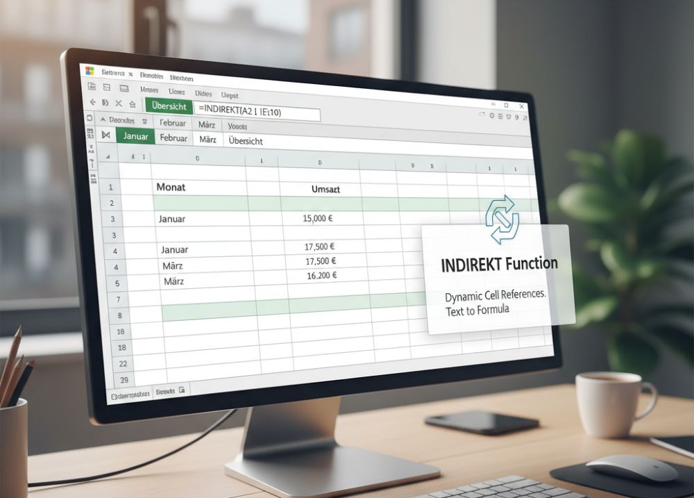
Mastering the INDIRECT function in Excel: Converting text into dynamic references
In the world of Excel, cell references like =A1 or =SUM(B2:B10) are commonplace. These references are direct and static. They always point to the same cell or range. But what if you want your reference to change based on the content of a different cell? That’s where the INDIRECT function comes in.
INDIRECT is a powerful, though often overlooked, function that takes a text string (plain text) and converts it into a real, working cell reference. It’s the tool of choice for making your spreadsheets dynamic and flexible.
What does the INDIRECT function do?
Imagine you have the text „B1“ in cell A1. If you then enter the formula =A1 in cell C1, the result is simply the text „B1“. However, if you enter the formula =INDIRECT(A1) in cell C1 instead, Excel looks at the content of A1 („B1“), converts this text into a reference to cell B1, and returns the value from cell B1.
INDIRECT thus acts as a translator: It reads a text string and tells Excel: „Hey, this isn’t normal text, this is an address. Go there and get the value.“
The Syntax Broken Down
The syntax of the function is relatively simple:
=INDIRECT(reference text; [A1])
Reference Text (Required): This is the text string that Excel should convert into a reference. This can be direct text (e.g., „C5“) or, much more commonly, a reference to a cell containing the text (e.g., A1). It can also be a formula that creates a text string (e.g., „Table“ & A2 & „!B5“).
[A1] (Optional): This argument specifies the reference type.
TRUE or omitted: Excel expects the default reference type „A1“ (e.g., B3, C4:D5).
FALSE: Excel expects the „R1C1“ reference type (Row 1 Column 1).
💡Tip: In 99% of cases, you can simply ignore and omit this argument.
Practical example: Dynamic data summarization
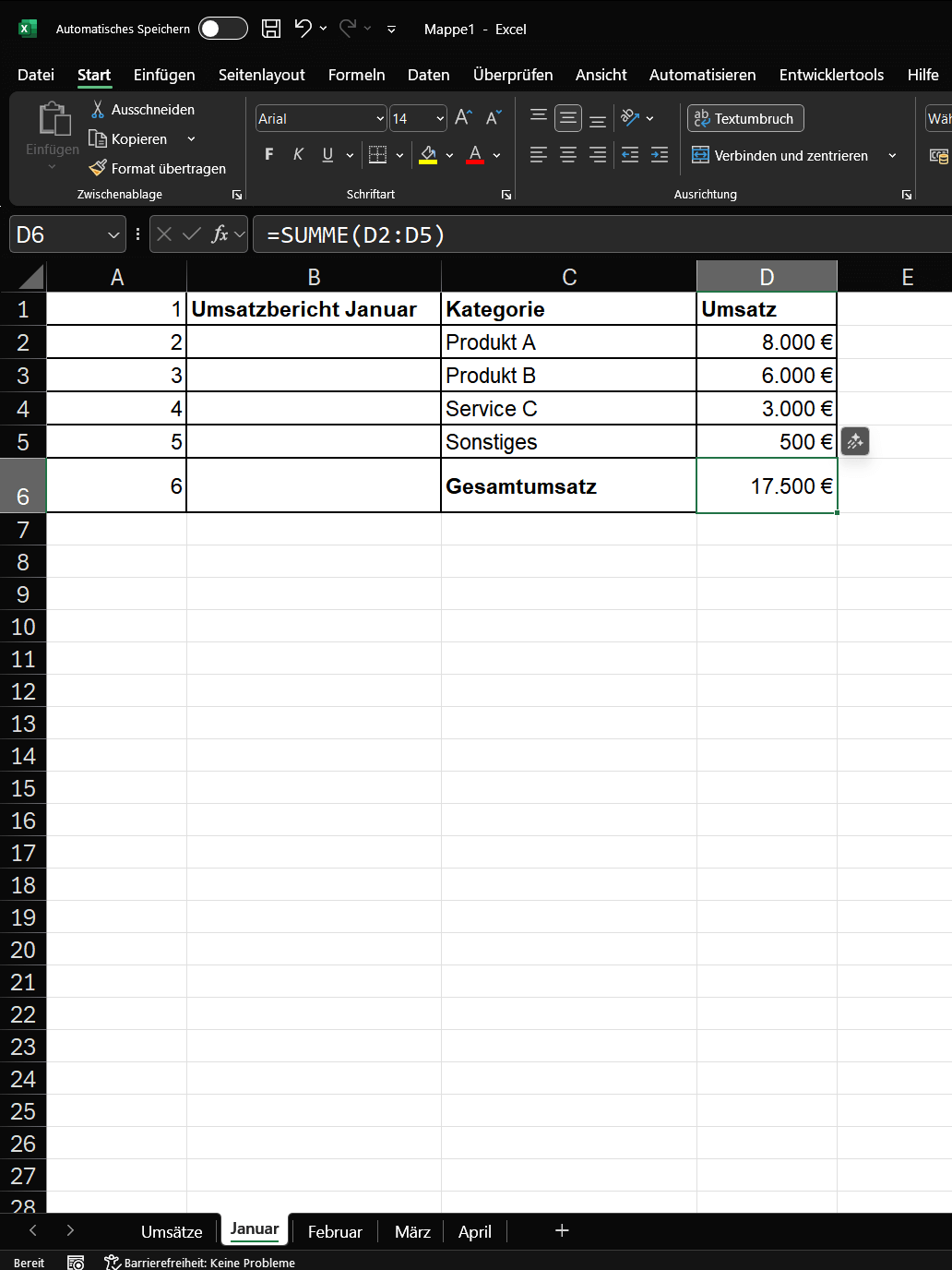
The best way to understand INDIRECT is through a practical example. Imagine you have a worksheet for each month of the year: „January,“ „February,“ „March,“ and so on.
In each of these monthly sheets, the total sales are in cell E10.
Now you want to create a summary table that lists all the total sales.
The slow, static way: In your summary table, you would manually type:
In B2: =January!D6
In B3: =February!D6
In B4: =March!D6
…and so on.
This is tedious and prone to errors. What if the cell changes? You would have to adjust all the formulas manually.
The fast, dynamic way with INDIRECT:
Set up your „Overview“ table so that the month names (which must be exactly the same as the worksheet names!) are in column A.
Set up your „Overview“ table so that the month names (which must be exactly the same as the worksheet names!) are in column A.
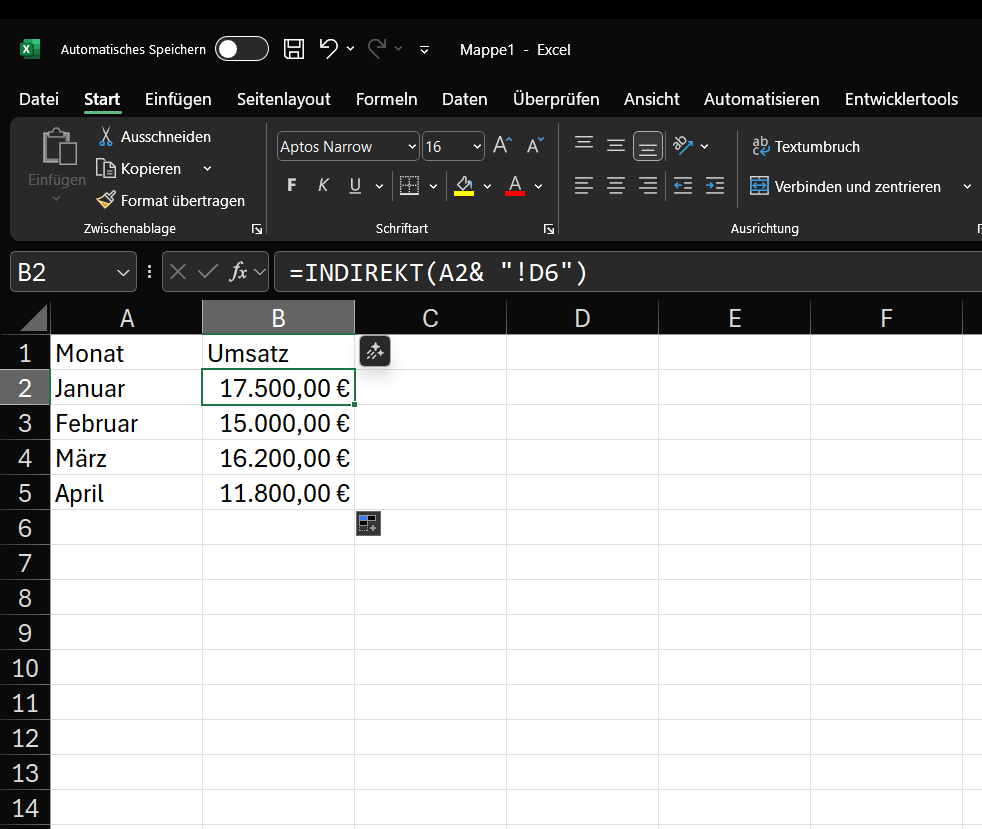
Go to cell B2 and enter the following formula:
=INDIRECT(A2 & „!D6“) [Cell D6 is just an example here. In your table, it must be named after the cell containing the desired value.]
Copy this formula down from B2 to B5.
What’s happening here?
- In cell B2:
- The formula takes the value from A2 („January“).
- It concatenates (&) it with the text string „!D6“.
- The result of this concatenation is the text: „January!D6“.
- INDIRECT takes this text and converts it into a real reference: January!D6.
- Excel retrieves the value from cell E10 of the „January“ sheet.
In cell B3 (when copying):
- The reference A2 automatically adjusts to A3.
- The formula is now =INDIRECT(A3 & „!D6“).
- It takes the value from A3 („February“) and creates the text „February!D6“.
- INDIRECT retrieves the value from cell D6 of the „February“ sheet.
You now have a single, flexible formula that you can use for all 12 months. If you add an „April“ sheet next year, you simply need to type „April“ in A5 and drag the formula down.
Why is the INDIRECT function so useful?
The main advantage of INDIRECT is its flexibility. It „decouples“ the formula from the actual reference. The reference is instead controlled by another cell’s content.
Other common use cases include:
- Dependent drop-down lists: You can create a drop-down list (data validation) whose options change depending on what is selected in another cell.
- Dynamic named ranges: You can reference a named range whose name is in a cell.
- Creating dashboards: You can control which data is displayed in a chart or table simply by changing a text value in a cell (e.g., „Week 1“, „Week 2“).
Important notes:
Despite its power, INDIRECT has two important drawbacks to be aware of:
- Volatileness: INDIRECT is a volatile function. This means it is recalculated whenever there is a change in the workbook, not just when its own input values change. In very large files with thousands of INDIRECT formulas, this can noticeably slow down Excel’s performance.
- Error vulnerability with references: If the reference text does not result in a valid reference (e.g., because the worksheet name was written „Jannuar“ instead of „January“), the function returns a #REF! error.
- Linked workbooks: If you use INDIRECT to reference another Excel file, that target file must be open for the reference to work.
Conclusion
The INDIRECT function is a powerful tool for advanced Excel users. It may seem complicated at first glance, but the concept is simple: it turns dead text into a living reference. If you ever reach a point where you think, „I wish my formula could adapt to the text in this cell,“ then INDIRECT is almost always the right answer.

Beliebte Beiträge

Word-Formatierungen endlich im Griff – Tutorial
Verzweifeln Sie nicht an zerschossenen Word-Dokumenten! Dieser Leitfaden zeigt Ihnen, wie Sie hartnäckige Formatierungen löschen, Formatvorlagen richtig nutzen und Steuerzeichen lesen. So sparen Sie Zeit und Nerven bei der Textverarbeitung.

Passwort für Word- und Excel-Dateien vergessen: So retten Sie Ihre Daten
Ein vergessenes Passwort bei Word oder Excel ist ärgerlich, bedeutet aber nicht immer Datenverlust. Während sich Schreibschutz durch einen XML-Trick umgehen lässt, erfordern verschlüsselte Dateien spezielle Tools. Hier finden Sie alle Lösungen im Überblick.

Excel KI-Update: So nutzen Sie Python & Copilot
Vergessen Sie komplexe Formeln! Excel wird durch Python und den KI-Copilot zum intelligenten Analysten. Diese Anleitung zeigt konkrete Beispiele, wie Sie Heatmaps erstellen, Szenarien simulieren und Ihre Arbeit massiv beschleunigen. Machen Sie Ihre Tabellen fit für die Zukunft.

Der XVERWEIS: Der neue Standard für die Datensuche in Excel
Verabschieden Sie sich vom Spaltenzählen! Der XVERWEIS macht die Datensuche in Excel endlich intuitiv und sicher. Erfahren Sie in diesem Tutorial, wie die Funktion aufgebaut ist, wie Sie sie anwenden und warum sie dem SVERWEIS und WVERWEIS haushoch überlegen ist.

Nie wieder Adressen abtippen: So erstellen Sie Serienbriefe in Word
Müssen Sie hunderte Briefe versenden? Schluss mit manuellem Abtippen! Erfahren Sie, wie Sie in wenigen Minuten einen perfekten Serienbrief in Word erstellen. Von der sauberen Excel-Datenbank bis zum fertigen Druck – unser Guide führt Sie sicher durch den Prozess.

Warum dein Excel-Kurs Zeitverschwendung ist – was du wirklich lernen solltest!
Hand aufs Herz: Wann hast du zuletzt eine komplexe Excel-Formel ohne Googeln getippt? Eben. KI schreibt heute den Code für dich. Erfahre, warum klassische Excel-Trainings veraltet sind und welche 3 modernen Skills deinen Marktwert im Büro jetzt massiv steigern.
Angebote 2025/2026 in: Vorlagen